
Problem: Define an ideal Fermi gas.
Solution: A non-interacting collection of identical fermions (e.g. electrons \(e^-\), neutrons \(n^0\), etc.). Mathematically, the “Fermi” part says that the state space is the antisymmetric submanifold \(\mathcal H=\bigwedge^NL^2(\mathbf R^3)\otimes\mathbf C^{2s+1}\) while the “ideal” part says that the Hamiltonian of the ideal Fermi gas does not contain any pairwise interaction potential \(V_{\text{int}}=0\) (note that “Pauli repulsion” or “exclusion pressure” mimics but is not an interaction):
\[H=\sum_{i=1}^N\frac{|\mathbf p_i|^2}{2m}+V_{\text{ext}}(\mathbf x_i)\]
Problem: Henceforth, assume \(V_{\text{ext}}=0\), so that \(H=T\) is purely kinetic. When it comes to analyzing the quantum statistics of the ideal Fermi gas, explain why it is advantageous to work in the grand canonical ensemble. Hence, obtain the Fermi-Dirac distribution \(\langle N_{|\mathbf k\rangle}\rangle\) of single-fermion \(|\mathbf k\rangle\)-state occupation numbers for an ideal Fermi gas.
Solution: Since \(H=T\) is purely kinetic, the \(H\)-eigenstates are just Slater determinants of distinct single-particle plane wave spinors \(\sqrt{N!}\mathcal A_N|\mathbf k_1,\sigma_1\rangle\otimes…\otimes|\mathbf k_N,\sigma_N\rangle\) where \(\langle\mathbf x|\mathbf k\rangle=e^{i\mathbf k\cdot\mathbf x}/\sqrt{V}\) with energy eigenvalues \(H\mathcal A_N|\mathbf k_1,\sigma_1\rangle\otimes…\otimes|\mathbf k_N,\sigma_N\rangle=\sum_{i=1}^N\frac{\hbar^2|\mathbf k_i|^2}{2m}\mathcal A_N|\mathbf k_1,\sigma_1\rangle\otimes…\otimes|\mathbf k_N,\sigma_N\rangle\).
If one were working in the canonical \((N,V,T)\) ensemble, evaluating the canonical partition function would require a sum over all \(N\)-fermion states of the form above which (if one actually takes a moment to think about it) is just a combinatorial nightmare to deal with (this is also not much better than asking how many \(N\)-fermion states there are with a given energy \(E\) as in the microcanonical \((N,V,E)\) ensemble). The upshot is that working in the grand canonical ensemble is ideal because one is then free to let \(N\) vary,
\[\mathcal Z=\prod_{|\mathbf k\rangle}\sum_{N_k=0,1}e^{-\beta(N_kE_k-\mu N_k)}=\prod_{|\mathbf k\rangle}\left(1+e^{-\beta(E_k-\mu)}\right)\]
From which the grand canonical potential is:
\[\Phi=-\frac{1}{\beta}\ln\mathcal Z=-\frac{1}{\beta}\sum_{|k\rangle\in\mathcal H_0}\ln\left(1+e^{-\beta(E_k-\mu)}\right)\]
And the average number of fermions is:
\[\langle N\rangle=-\frac{\partial\Phi}{\partial\mu}=\sum_{|k\rangle\in\mathcal H_0}\frac{1}{e^{\beta(E_k-\mu)}+1}\]
from which one immediately reads off the Fermi-Dirac distribution of the Fermi occupation numbers of each of the single-fermion states \(|k\rangle\):
\[\langle N_k\rangle=\frac{1}{e^{\beta(E_k-\mu)}+1}\]
It is remarkable that a mere sign change in the denominator from the Bose-Einstein distribution is all that is needed to enforce the Pauli exclusion principle. Unlike for the ideal Bose gas where the chemical potential \(\mu<0\) had to be negative, for the Fermi-Dirac distribution \(\mu\in\textbf R\) can be anything.
Just as with the ideal Bose gas, for an ideal Fermi gas one would like to approximate the series with integrals (called the Thomas-Fermi approximation) \(\sum_{|k\rangle\in\mathcal H_0}\mapsto\int_0^{\infty}g(E)dE\). Taking the ideal Fermi gas to be non-relativistic, one has the density of states:
\[g(E)=\frac{g_sm^{3/2}V}{\sqrt{2}\pi^2\hbar^3}\sqrt{E}\]
where \(g_s=2s+1\) is a spin degeneracy factor (which has to be explicitly included for fermions by virtue of the spin-statistics theorem \(s=1/2,3/2,5/2,…\) and the fact that the free Hamiltonian \(H=T\) commutes with \(\textbf S^2\)). In the grand canonical ensemble, one thus has for an ideal Fermi gas:
\[\Phi=\frac{g_sV}{\beta\lambda^3}\text{Li}_{5/2}(-z)\]
\[\langle N\rangle=-\frac{g_sV}{\lambda^3}\text{Li}_{3/2}(-z)\]
\[\langle E\rangle=-\frac{3g_sV}{2\beta\lambda^3}\text{Li}_{5/2}(-z)\]
from which one obtains \(pV=\frac{2}{3}E\) for an ideal Fermi gas as was the case for the ideal Bose gas (and the ideal classical gas). In the high-temperature \(T\to\infty\) limit \(z\to 0\), one finds that, similar to the ideal Bose gas, the ideal Fermi gas looks like an ideal classical gas, at least to first order in the virial expansion (at second order, the quantum correction actually increases the pressure of the ideal Fermi gas whereas it was decreasing for the ideal Bose gas):
\[pV=NkT\left(1+\frac{\lambda^3N}{4\sqrt{2}g_sV}+O\left(\frac{N}{V}\right)^2\right)\]
In order to see more interesting, non-classical physics, it will as usual be necessary to look in the low-temperature limit \(T\to 0,z\to 1\). In fact, to start, one may as well look directly at the case of absolute zero \(T=0\). In this case, the ideal Fermi gas is said to be degenerate. At a glance, this is because the Fermi-Dirac distribution for the Fermi occupation numbers reduces to a top-hat filter:
\[N_k=\frac{1}{e^{\beta(E_k-\mu)}+1}=[E_k<\mu]\]
One can define the Fermi energy by \(E_F:=\mu(T=0)\) so that states \(|k\rangle\) with \(\hbar^2k^2/2m<E_F\) lying in the Fermi sea are fully occupied (i.e. have Fermi occupation number of \(N_k=1\)) while states \(|k\rangle\) with \(\hbar^2k^2/2m>E_F\) lying beyond the Fermi surface are completely empty. This definition of the Fermi energy \(E_F\) is strictly speaking a bit misleading since in the grand canonical ensemble \(\mu\) and \(T\) are independent and fixed while \(N\) fluctuates; in practice \(N\) is fixed and both \(\mu\) and \(T\) fluctuate in a way to keep \(N\) fixed so that working in the grand canonical ensemble is just a mathematical convenience. Therefore, it would make more sense to express/define \(E_F\) in terms of the fixed number \(N\) of fermions in the degenerate ideal Fermi gas:
\[N=\sum_{|k\rangle\in\mathcal H_0}N_k=\int_0^{\infty}[E<E_F]g(E)dE=\int_0^{E_F}g(E)dE\Rightarrow E_F=\frac{\hbar^2}{2m}\left(\frac{6\pi^2 N}{g_sV}\right)^{2/3}\]
This is of course related to the Fermi momentum and Fermi temperature by \(E_F=\hbar^2k_F^2/2m=kT_F\). The Fermi temperature \(T_F\) for the ideal Fermi gas determines whether the ideal Fermi gas is in the high-temperature \(T>T_F\) regime or the low-temperature \(T<T_F\) regime. For example, in a copper \(\text{Cu(s)}\) wire the number density of electrons \(e^-\) is \(N/V\approx 8.5\times 10^{28}\text{ m}^{-3}\), so the corresponding Fermi temperature is actually quite hot \(T_F\approx 8.2\times 10^4\text{ K}\) by everyday standards, and so in particular room temperature \(T\approx 300\text{ K}\ll T_F\) means that the electrons \(e^-\) in metals can be thought of to a good approximation as degenerate \(T=0\) Fermi gases.
Having computed the total number of fermions \(N=\langle N\rangle\), one can also compute the total energy \(E=\langle E\rangle\) in the grand canonical ensemble:
\[E=\sum_{|k\rangle\in\mathcal H_0}N_kE_k=\int_0^{\infty}[E<E_F]Eg(E)dE=\int_0^{E_F}Eg(E)dE=\frac{3}{5}NE_F\]
which is pretty intuitive, the factor of \(3/5\) essentially just coming from the average of \(k^2\) in a ball of radius \(k_F\), i.e. \(\frac{3}{4\pi k_F^3}\int_0^{k_F}k^24\pi k^2dk=\frac{3}{5}k_F^2\).
Finally, the “equation of state” \(pV=\frac{2}{3}E\) earlier yields the corresponding degeneracy pressure:
\[pV=\frac{2}{5}NE_F\]
For comparison, recall that below the critical temperature \(T<T_c\) the pressure \(p\sim T^{5/2}\) of a BEC approached \(p\to 0\) as \(T\to 0\); not so for an ideal Fermi gas. For both the ideal Bose and Fermi gases, \(pV=\frac{2}{3}E\) but because bosons can condense to the \(E=0\) ground state, their pressure \(p\) also drops to \(p\to 0\), however fermions cannot do this because of the Pauli exclusion principle (they are forced to fill out a Fermi sea instead), so their total energy \(E=\frac{3}{5}NE_F\) can never reach zero, and therefore their pressure \(p\) also cannot reach \(p\to 0\), leaving this residual \(T=0\) degeneracy pressure \(p=\frac{2}{5}\frac{N}{V}E_F>0\).
Finally, it is worth asking more generally just about the physics of an ideal Fermi gas not necessarily when it is degenerate at \(T=0\), but merely at some “low” temperature \(T\ll T_F\). Here, “physics” shall mean “low-temperature heat capacity” \(C_V=C_V(T)\).
In this case, the Fermi-Dirac distribution will be distorted from the degenerate \(T=0\) top-hat filter into a distribution that looks like:
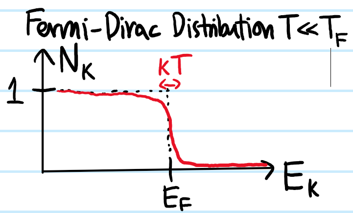
The key observation is that only fermions close to the Fermi surface, specifically whose energy is within \(kT\) of the Fermi energy \(E_F\) can respond to any additional energy added to the ideal Fermi gas, and therefore contribute to the heat capacity \(C_V\) (since only they notice the non-degenerate temperature \(T>0\), the rest of the fermions being locked in the Fermi sea by the Pauli exclusion principle).
\[C_V=\frac{\partial E}{\partial T}=-\frac{3g_sV}{2}\frac{\partial}{\partial T}\left(\frac{1}{\beta\lambda^3}\text{Li}_{5/2}(-z)\right)\]
At this point, invoke the behavior of the polylogarithm as the fugacity \(z\to 1\) in the low-\(T\) limit (called the Sommerfeld expansion, essentially just a lot of binomial expansions):
\[-\text{Li}_{s}(-z)=\frac{(\ln z)^s}{\Gamma(s+1)}\left(1+\frac{\pi^2}{6}\frac{s(s-1)}{(\ln z)^2}+…\right)\]
where \(\ln z=\beta\mu\), so this simplifies to:
\[C_V\approx \frac{\sqrt{2}g_sm^{3/2}V}{5\pi^2\hbar^3}\frac{\partial}{\partial T}\left(\mu^{5/2}\left(1+\frac{5\pi^2}{8\beta^2\mu^2}\right)\right)\]
Problem: Explain why, in order for the number of fermions \(N\) in the gas to be fixed, in particular \(dN/dT=0\), the chemical potential \(\mu\) must become a function of temperature \(\mu=\mu(T)\).
Solution: Simply because:
\[N=\int_0^{\infty}dEg(E)\frac{1}{e^{\beta(E-\mu)}+1}\]
So if the LHS is a constant, but the RHS has an explicit \(T\)-dependence in the \(\beta=1/k_BT\), so \(\mu(T)\) must vary implicitly so as to “offset” the explicit \(T\) variation in \(\beta\) to keep the overall integral constant.
Problem: At \(T=0\), the value of the chemical potential is by definition called the Fermi energy \(E_F:=\mu(T=0)\) of the Fermi gas, i.e. roughly speaking each additional fermion added to the gas increases the gas’s energy by \(E_F\) since that fermion would be added to the Fermi surface. State how \(E_F\) scales with the number density \(N/V\) of fermions in the gas in dimension \(d\).
Solution: The key point to realize is that at \(T=0\) the Fermi-Dirac distribution becomes a step function \([E<E_F]\), so one has the implicit equation for \(E_F\):

So in particular, the important point to remember is that \(E_F\sim (N/V)^{2/d}\).
Problem: Now suppose, instead of working with a strictly degenerate \(T=0\) Fermi gas, one heats the gas up a little to some strictly positive temperature \(T>0\), but still much less than the gas’s Fermi temperature \(T_F:=E_F/k_B\). In this low-\(T\) regime, use the Sommerfeld expansion to show that the chemical potential \(\mu(T)\) decreases (provided \(d\geq 3\)) quadratically from its \(T=0\) value of \(\mu(T=0)=E_F\), in particular \(\partial\mu/\partial T|_{T=0}=0\) so to \(1^{\text{st}}\)-order provided \(T\ll T_F\) one can often get away with approximating the chemical potential \(\mu\approx E_F\) by its constant value at \(T=0\).
Solution:


A comment: recall that the Bose-Einstein distribution \(\frac{1}{e^{\beta(E-\mu)}-1}\) comes from summing a suitable geometric series in the partition function. The idea of the Sommerfeld expansion is kinda to undo this step, recasting distribution back into its geometric series form…except the catch here is that one is working with the Fermi-Dirac distribution, not the Bose-Einstein, and indeed in the derivation of the Fermi-Dirac distribution there was no geometric series involved (or a trivial geometric series of just \(2\) terms if one likes), yet the way the sum is being unwrapped is more in the spirit of Bose-Einstein statistics…is there any connection here or just a mere mathematical coincidence?
Finally, it is clear that one can re-express the heat capacity in terms of \(N\) and \(E_F\) (the fixed variables) as:
\[C_V=\frac{3N}{5}\frac{\partial}{\partial T}\left(\mu\frac{1+5\pi^2k^2T^2/8\mu^2}{1+\pi^2k^2T^2/8\mu^2}\right)\approx\frac{3NE_F}{5}\frac{\partial}{\partial T}\left(1-\left(\frac{5}{8}-\frac{1}{8}-\frac{1}{12}\right)\frac{\pi^2}{\beta^2E_F^2}\right)\]
leading to the linear heat capacity behavior of the low-\(T\) ideal Fermi gas:
\[C_V=\frac{\pi^2}{2}Nk\frac{T}{T_F}\]
Ignoring the \(\pi^2/2\) prefactor which came from the detailed Sommerfeld expansion of the polylogarithms, there is a simple intuitive way to understand this formula: the number of Fermi surface fermions living within \(kT\) of the Fermi energy \(E_F\) is \(g(E_F)kT\) and the energy of each fermion is of order \(kT\) so the total energy of all Fermi surface fermions is \(E\sim g(E_F)(kT)^2\). If one adds some energy \(dE\) into the ideal Fermi gas, then essentially all this energy has to go into the Fermi surface fermions so that one may legitimately equate \(dE\sim g(E_F)k^2TdT\) reproducing the linear heat capacity:
\[C_V\sim g(E_F)k^2T\sim E_F^{1/2}k^2T\sim N^{1/3}k^2T\sim Nk\frac{T}{T_F}\]
Actually, even the pre-factor \(\pi^2/2\) from the Sommerfeld expansion can almost be calculated correctly. Since \(N=\int_0^{E_F}dEg(E)\) and the integral of a power \(g(E)\sim E^{1/2}\) is just \(N=\frac{2}{3}E_Fg(E_F)\), and since this is basically a free electron gas (minus Pauli as usual), any injection of energy goes directly into Fermi surface electrons. There are \(g(E_F)k_BT\) of these states, which, assuming they’re all completely filled, also means there are that many electrons, each with the equipartition kinetic energy \(3k_BT/2\):
\[dE=g(E_F)k_BT\times\frac{3}{2}k_BT\]
so \(C_V=\partial _TE=\frac{9}{2}Nk_B\frac{T}{T_F}\).
A more visually intuitive way to understand how \(\mu\) depends on \(T\):

The theory of ideal Fermi gases has diverse applications, ranging from electrons \(e^-\) in a conductor (as justified by Landau’s Fermi liquid theory) to astrophysics (e.g. white dwarf stars are supported by electron degeneracy pressure, neutron stars are supported by neutron degeneracy pressure, thanks to the fact that both electrons \(e^-\) and neutrons \(n^0\) are fermions) to Pauli paramagnetism and Landau diamagnetism in condensed matter physics.