
The purpose of this post is to appreciate that the familiar idea of non-interacting particles from e.g. statistical mechanics manifests in the context of QFT as a free quantum field theory.
Problem #\(1\): What defines a free classical field theory? Give an example.
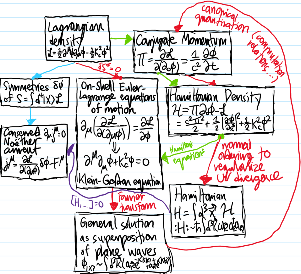
Solution #\(1\): A classical field theory is said to be free iff its Lagrangian density \(\mathcal L\), or equivalently Hamiltonian density \(\mathcal H\), is quadratic in all fields \(\phi_i\). Why? Because the corresponding Euler-Lagrange equations of motion for the fields \(\phi_i\) would then be linear in the \(\phi_i\). An example of a free classical field theory is the classical Klein-Gordon field theory which governs just a single, relativistic, real scalar field \(\phi(X)\):
\[\mathcal L=\frac{1}{2}\partial^{\mu}\phi\partial_{\mu}\phi-\frac{1}{2}k_c^2\phi^2\]
\[\mathcal H=\frac{c^2\pi^2}{2}+\frac{1}{2}\biggr|\frac{\partial\phi}{\partial\textbf x}\biggr|^2+\frac{1}{2}k_c^2\phi^2\]
\[\partial^{\mu}\partial_{\mu}\phi+k_c^2\phi=0\]
(aside: Klein-Gordon field theory is “relativistic” in the sense of being Lorentz-invariant as manifest from the Lagrangian density \(\mathcal L\). It is “real” \(\phi(X)\in\textbf R\) because, when canonically quantized, it turns out to only give rise to neutral particles. It is clearly free. And it is a scalar field (as opposed to a vector field like in E&M) because, again when canonically quantized from a CFT to a QFT, turns out to also only describe spinless \(s=0\) bosons). Think Higgs boson for instance.
Problem #\(2\): In the context of the quantum harmonic oscillator from non-relativistic particle mechanics, the operators \(a,a^{\dagger}\) are typically called lowering and raising operators respectively. In moving from quantum particles to quantum fields however, the key conceptual leap that the number of particles is not conserved gives rise to an entirely new perspective on what \(a,a^{\dagger}\) are so that in QFT they are called annihilation and creation operators.
But, first, just using “classical cheating”, define \(a\) and \(a^{\dagger}\) and compute their commutator \([a,a^{\dagger}]\). Also define the number operator \(N\) and compute \([N,a]\) and \([N,a^{\dagger}]\).
Solution #\(2\): By inspecting the classical Hamiltonian:
\[H(x,p)=\frac{p^2}{2m}+\frac{m\omega^2x^2}{2}\]
One can construct a characteristic quantum oscillator length \(x_0\) and oscillator momentum \(p_0\) through the virial relations:
\[\frac{\hbar\omega}{2}=\frac{p_0^2}{2m}=\frac{m\omega^2x_0^2}{2}\]
So that:
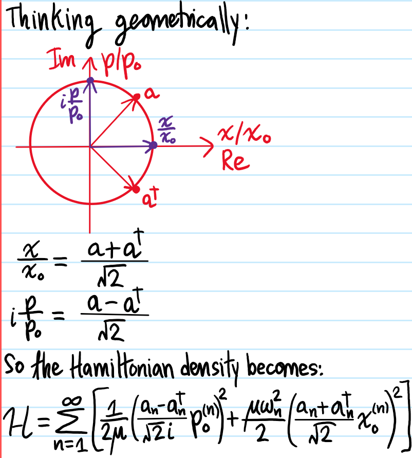
\[H=\frac{\hbar\omega}{2}\left(\left(\frac{x}{x_0}\right)^2+\left(\frac{p}{p_0}\right)^2\right)\]
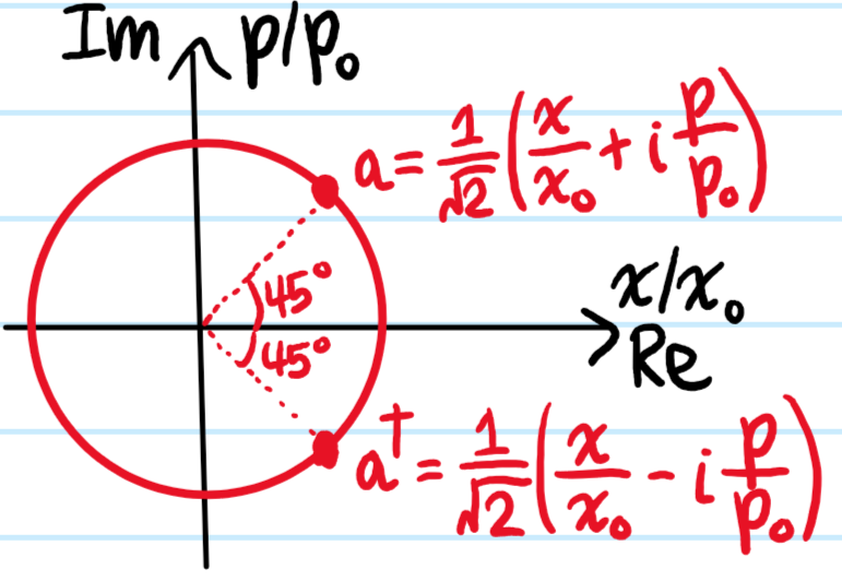
This sum of squares suggests the classical factorization:
\[H=\hbar\omega N\]
where \(N:=aa^{\dagger}\) and the isomorphism \(\cong\) between phase space \(\textbf R^2\) and the complex plane \(\textbf C\) is exploited:
Since canonical quantization is a Lie algebra representation up to quadratic polynomials on phase space (which applies to everything here), it follows that all Poisson bracket computations must agree with the corresponding commutators. In particular:
\[\{a,a^{\dagger}\}=\det\begin{pmatrix}\partial a/\partial x&\partial a^{\dagger}/\partial x \\ \partial a/\partial p & \partial a^{\dagger}/\partial p\end{pmatrix}=-\frac{i}{x_0p_0}=\frac{1}{i\hbar}\]
which could also be obtained just from drawing pictures like:
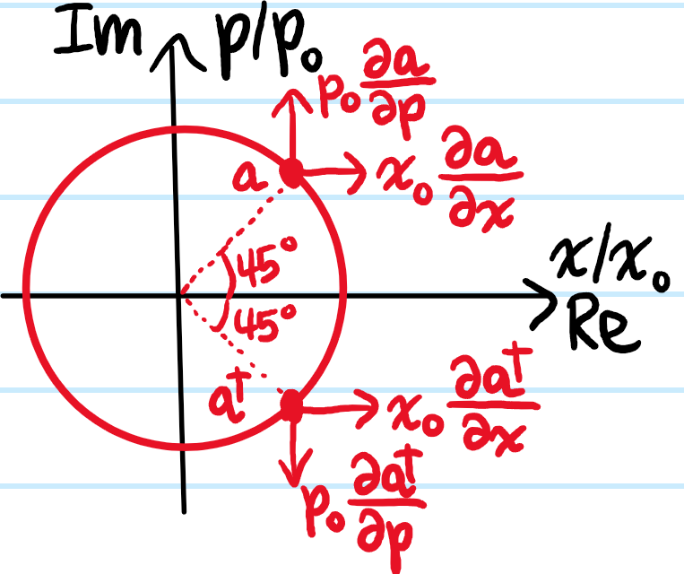
This “proves” that \([a,a^{\dagger}]=i\hbar\{a,a^{\dagger}\}=1\). The other commutators can be quickly obtained using the “product rule” for Poisson brackets:
\[\{N,a\}=\{aa^{\dagger},a\}=a\{a^{\dagger},a\}+\{a,a\}a^{\dagger}=-\frac{a}{i\hbar}\Rightarrow [N,a]=-a\]
\[\{N,a^{\dagger}\}=\{N,a\}^{\dagger}=\frac{a^{\dagger}}{i\hbar}\Rightarrow [N,a^{\dagger}]=a^{\dagger}\]
(note that although \([F,G]^{\dagger}=[G^{\dagger},F^{\dagger}]\) for commutators, for Poisson brackets it’s just \(\{f,g\}^{\dagger}=\{f^{\dagger},g^{\dagger}\}\)).
Problem #\(3\): A \(1\)D string has Hamiltonian density:
\[\mathcal H=\sum_{n=1}^{\infty}\left(\frac{p_n^2}{2\mu}+\frac{1}{2}\mu\omega_n^2x_n^2\right)\]
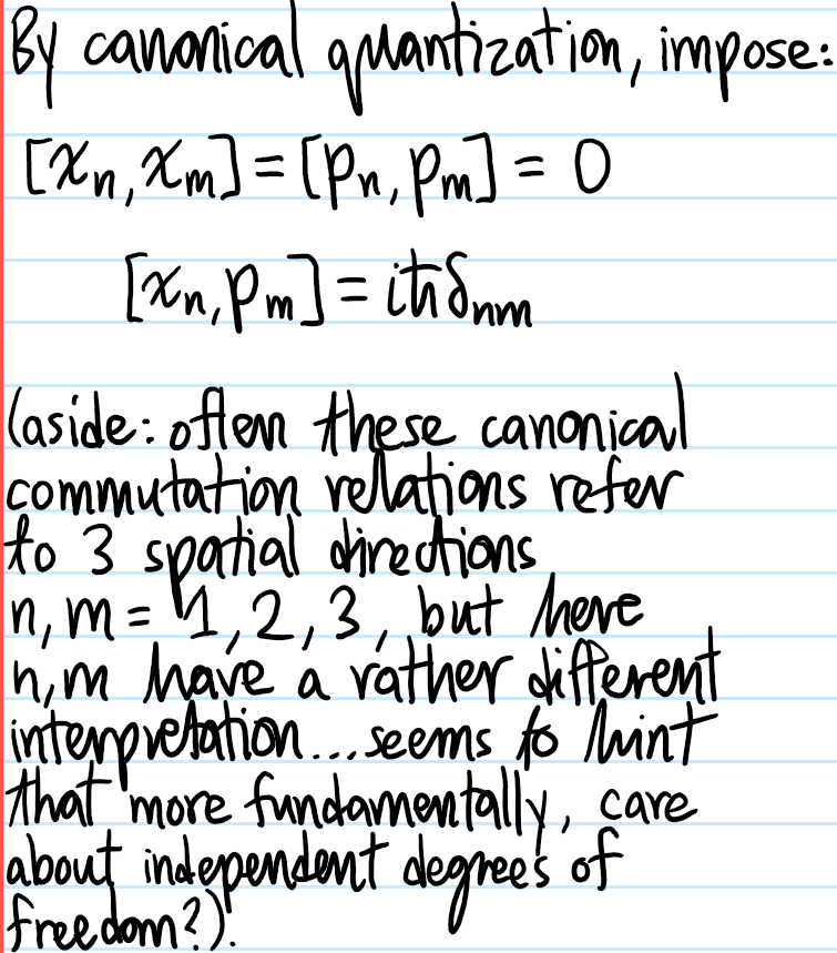
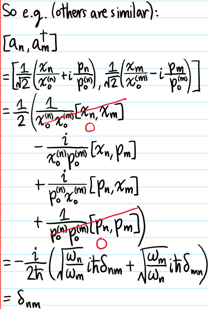
Unlike the previous problem where there was just \(1\) harmonic oscillator, here there are an infinite number of harmonic oscillators, one for each normal mode \(n=1,2,3,…\) (however, here it is only countably infinite; in QFT it will often be uncountably infinite!). Thus, each one gets its own pair of creation and annihilation operators \(a_n,a_n^{\dagger}\) defined analogously as in Problem #\(2\) (but where each oscillator now also has its own characteristic length \(x_0^{(n)}=\sqrt{\hbar/\mu\omega_n}\) and characteristic momentum \(p_0^{(n)}=\sqrt{\hbar\mu\omega_n}\)). Check that for distinct oscillators \(n\neq m\), these operators don’t talk to each other in the sense that \([a_n,a_m]=[a_n^{\dagger},a_m^{\dagger}]=0\) and \([a_n,a_m^{\dagger}]=\delta_{nm}\). Show that the Hamiltonian density can be rewritten:
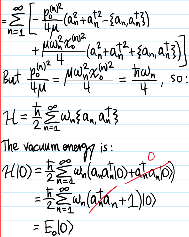
\[\mathcal H=\frac{\hbar}{2}\sum_{n=1}^{\infty}\omega_n\{a_n,a_n^{\dagger}\}\]
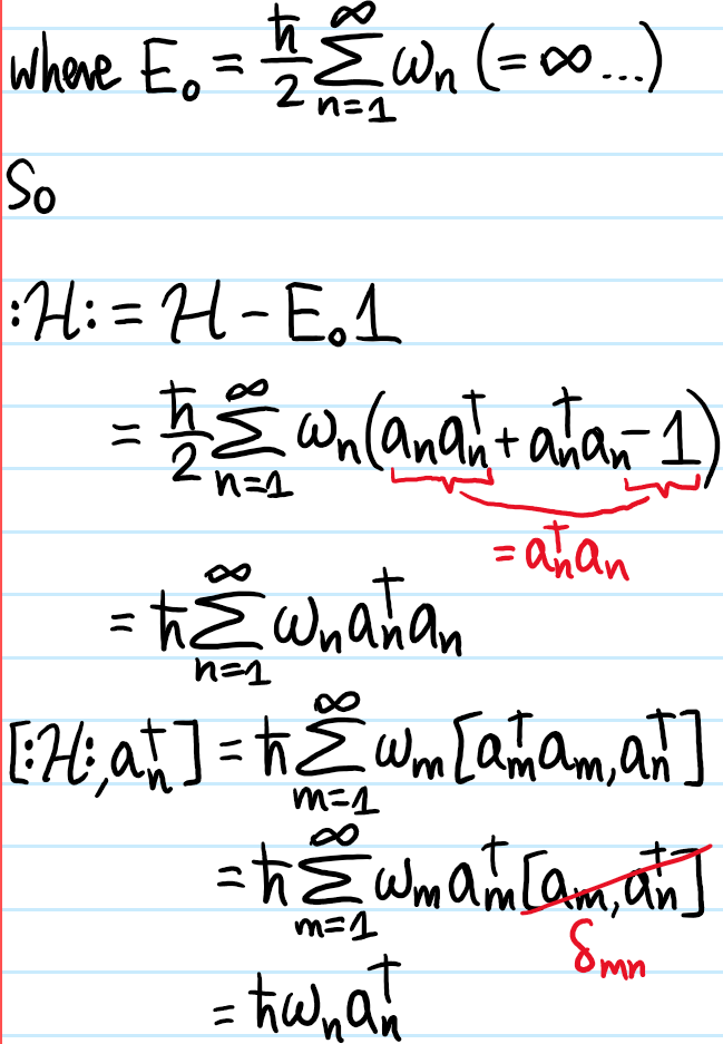
Assuming there exists a single universal ground state \(|0\rangle\) annihilated by \(a_n|0\rangle=0\) for all \(n=1,2,3,…\), show that, after discarding the vacuum energy, \(\mathcal H\mapsto :\mathcal H:\) takes the normally ordered form:
\[:\mathcal H:=\hbar\sum_{n=1}^{\infty}\omega_na_n^{\dagger}a_n\]
And also show that \([:\mathcal H:,a_n^{\dagger}]=\hbar\omega_na_n^{\dagger}\). Hence calculate the energy of the excited Fock state:
\[|N_1,N_2,…,N _n\rangle=(a_1^{\dagger})^{N_1}(a_2^{\dagger})^{N_2}…(a_n^{\dagger})^{N_n}|0\rangle\]
Solution #\(3\):
Problem #\(4\): What is the most general real scalar field solution of the classical Klein-Gordon equation?
Solution #\(4\): Since it’s a linear PDE, it makes sense to change to the Fourier basis for the real scalar field:
\[\phi(\textbf x,t)=\frac{1}{(2\pi)^{3/2}}\int\hat{\phi}(\textbf k,t)e^{i\textbf k\cdot\textbf x}d^3\textbf k\]
Substituting this as an ansatz into the Klein-Gordon equation yields, for each \(\textbf k\in\textbf R^3\), the equation of motion of a simple harmonic oscillator for \(\hat{\phi}(\textbf k,t)\):
\[\frac{\partial^2\hat{\phi}}{\partial t^2}+\omega_{\textbf k}^2\hat{\phi}=0\]
where the relativistic dispersion relation for the oscillator frequency is:
\[\omega_{\textbf k}=c\sqrt{|\textbf k|^2+k_c^2}\]
(defined here as the positive square root). So the most general solution in \(\textbf k\)-space is parameterized by two arbitrary scalar fields \(a_{\textbf k},b_{\textbf k}\):
\[\hat{\phi}(\textbf k,t)=a_{\textbf k}e^{-i\omega_{\textbf k}t}+b_{\textbf k}e^{i\omega_{\textbf k}t}\]
leading to the corresponding general solution in \(\textbf x\)-space:
\[\phi(\textbf x,t)=\frac{1}{(2\pi)^{3/2}}\int\left(a_{\textbf k}e^{i(\textbf k\cdot\textbf x-\omega_{\textbf k}t)}+b_{\textbf k}e^{i(\textbf k\cdot\textbf x+\omega_{\textbf k}t)}\right)d^3\textbf k\]
However, demanding that \(\phi(\textbf x,t)\) be a real scalar field so that \(\phi^{\dagger}(\textbf x,t)=\phi(\textbf x,t)\) (which is equivalent to demanding that its Fourier transform be Hermitian \(\hat{\phi}^{\dagger}(\textbf k,t)=\hat{\phi}(-\textbf k,t)\)) forces \(b_{\textbf k}=a_{-\textbf k}^{\dagger}\). Thus actually one can simply write:
\[\phi(\textbf x,t)=\frac{1}{(2\pi)^{3/2}}\int\left(a_{\textbf k}e^{i(\textbf k\cdot\textbf x-\omega_{\textbf k}t)}+a_{\textbf k}^{\dagger}e^{-i(\textbf k\cdot\textbf x-\omega_{\textbf k}t)}\right)d^3\textbf k\]
Or, defining the four-wavevector \(|K\rangle:=(\omega_{\textbf k}/c, \textbf k)\), working with the standard four-position \(|X\rangle:=(ct,\textbf x)\), and using the time-like convention for the Minkowski metric \(\eta=\text{diag}(1,-1,-1,-1)\):
\[\phi(X)=\frac{1}{(2\pi)^{3/2}}\int\left(a_{\textbf k}e^{-i\langle K|X\rangle}+a_{\textbf k}^{\dagger}e^{i\langle K|X\rangle}\right)d^3\textbf k\]
Note here that one is still working entirely within the realm of classical field theory (not QFT yet!) so the daggers \(\dagger\) are nothing more than complex conjugation, and in particular \(\phi(X)\) is a (real) scalar field rather than a (Hermitian) operator field. This is similarly the case with \(a_{\textbf k},a_{\textbf k}^{\dagger}\) being (complex) scalar fields at this stage rather than operator fields. Finally, it is worth noting that the conjugate real scalar momentum field is:
\[\pi(X):=\frac{1}{c^2}\frac{\partial\phi}{\partial t}=\frac{-i}{(2\pi)^{3/2}c^2}\int\omega_{\textbf k}\left(a_{\textbf k}e^{-i\langle K|X\rangle}-a_{\textbf k}^{\dagger}e^{i\langle K|X\rangle}\right)d^3\textbf k\]
Problem #\(5\): As warmup for the next problem, evaluate the Fourier transform of the plane wave with wavevector \(\textbf k_0\):
\[\frac{1}{(2\pi)^{3/2}}\int e^{i(\textbf k_0\cdot\textbf x-\omega t)}e^{-i\textbf k\cdot\textbf x}d^3\textbf x\]
Solution #\(5\): Under this unitary convention for the Fourier transform, it is:
\[\frac{1}{(2\pi)^{3/2}}\int e^{i(\textbf k_0\cdot\textbf x-\omega t)}e^{-i\textbf k\cdot\textbf x}d^3\textbf x=(2\pi)^{3/2}\delta^3(\textbf k-\textbf k_0)e^{-i\omega t}\]
As one may check by computing the “inverse Fourier transform” and using the non-negotiable, defining sifting property of the \(\delta\)-distribution:
\[\frac{1}{(2\pi)^{3/2}}\int (2\pi)^{3/2}\delta^3(\textbf k-\textbf k_0)e^{-i\omega t}e^{i\textbf k\cdot\textbf x}d^3\textbf k=e^{i(\textbf k_0\cdot\textbf x-\omega t)}\]
Problem #\(6\): Explain what it means to take the classical Klein-Gordon theory governing the real scalar fields \(\phi(X),\pi(X)\) and canonically quantize them in the Heisenberg picture to Hermitian operator fields, thereby constructing a free quantum Klein-Gordon field theory. What changes in the Schrodinger picture?
Solution #\(6\): On paper, the equations are invariant. Canonical quantization is really more of a conceptual leap, in that the fundamental “data type” of the objects in the equations are what changes. Specifically, one now promotes \(\phi(X),\pi(X)\) to operator fields, i.e. a function associating an operator to each event \(|X\rangle\) in Minkowski spacetime. It follows that the only way the classical Klein-Gordon field decompositions in the Fourier basis of plane waves can be compatible with canonical quantization is iff, in addition to promoting \(\phi(X),\pi(X)\) to operator fields, one also/simultaneously promotes the “Fourier coefficients” \(a_{\textbf k},a_{\textbf k}^{\dagger}\) to operators.
Furthermore, it turns out one should postulate equal-\(t\) commutation relations between these operators in the Heisenberg picture:
\[[\phi(\textbf x,t),\phi(\textbf x’,t)]=[\pi(\textbf x,t),\pi(\textbf x’,t)]=0\]
\[[\phi(\textbf x,t),\pi(\textbf x’,t)]=i\hbar\delta^3(\textbf x-\textbf x’)\]
though one can show through straightforward computations in the spirit of Problem #\(5\) that these are logically equivalent to the following commutation relations on the Fourier coefficients (cf. Problem #\(3\)):
\[[a_{\textbf k},a_{\textbf k’}]=[a_{\textbf k}^{\dagger},a_{\textbf k’}^{\dagger}]=0\]
\[[a_{\textbf k},a_{\textbf k’}^{\dagger}]=\frac{\hbar c^2}{2\omega_{\textbf k}}\delta^3(\textbf k-\textbf k’)\]
(note other normalization conventions also exist). For example:
\[\hat{\pi}(\textbf k,t)=\frac{1}{(2\pi)^{3/2}}\int d^3\textbf x e^{-i\textbf k\cdot\textbf x}\frac{-i}{(2\pi)^{3/2}c^2}\int\omega_{\textbf k’}\left(a_{\textbf k’}e^{-i\langle K’|X\rangle}-a_{\textbf k’}^{\dagger}e^{i\langle K’|X\rangle}\right)d^3\textbf k’\]
\[=-\frac{i}{(2\pi)^3c^2}\int d^3\textbf k’ d^3\textbf x\omega_{\textbf k’}\left(a_{\textbf k’}e^{i(\textbf k’-\textbf k)\cdot\textbf x}e^{-i\omega_{\textbf k’}t}-a_{\textbf k’}^{\dagger}e^{-i(\textbf k’+\textbf k)\cdot\textbf x}e^{i\omega_{\textbf k’}t}\right)\]
\[=-\frac{i}{(2\pi)^3c^2}\int d^3\textbf k’\omega_{\textbf k’}\left(a_{\textbf k’}(2\pi)^3\delta^3(\textbf k’-\textbf k)e^{-i\omega_{\textbf k’}t}-a_{\textbf k’}^{\dagger}(2\pi)^3\delta^3(\textbf k+\textbf k’)e^{i\omega_{\textbf k’}t}\right)\]
\[=-\frac{i\omega_{\textbf k}}{c^2}(a_{\textbf k}e^{-i\omega_{\textbf k}t}-a^{\dagger}_{-\textbf k}e^{i\omega_{\textbf k}t})\]
where the isotropy of the dispersion relation \(\omega_{-\textbf k}=\omega_{\textbf k}=\omega_{|\textbf k|}\) has been used. The expression for \(\hat{\phi}(\textbf k,t)\) was already given above, but can also of course be recovered by identical manipulations. So, in analogy with the classical case in Problem #\(3\), one has:
\[a_{\textbf k}=\frac{e^{i\omega_{\textbf k}t}}{2}\left(\hat{\phi}(\textbf k,t)+\frac{ic^2}{\omega_{\textbf k}}\hat{\pi}(\textbf k,t)\right)\]
\[a_{-\textbf k}^{\dagger}=\frac{e^{-i\omega_{\textbf k}t}}{2}\left(\hat{\phi}(\textbf k,t)-\frac{ic^2}{\omega_{\textbf k}}\hat{\pi}(\textbf k,t)\right)\]
which are happily consistent with each other (note also that \(a_{\textbf k}\) is \(t\)-independent so all \(t\)-dependence on the right-hand side is spurious). One then has e.g.
\[[a_{\textbf k},a_{\textbf k’}^{\dagger}]=\frac{e^{i(\omega_{\textbf k}-\omega_{\textbf k’})t}}{4}\left([\hat{\phi}(\textbf k,t),\hat{\phi}(-\textbf k,t)]+\frac{ic^2}{\omega_{\textbf k}}[\hat{\pi}(\textbf k,t),\hat{\phi}(-\textbf k’,t)]-\frac{ic^2}{\omega_{\textbf k}}[\hat{\phi}(\textbf k,t),\hat{\pi}(-\textbf k’,t)]+\frac{c^4}{\omega_{\textbf k}\omega_{\textbf k’}}[\hat{\pi}(\textbf k,t),\hat{\pi}(-\textbf k’,t)]\right)\]
But the commutation relations postulated on \(\phi(\textbf x,t)\) and \(\pi(\textbf x,t)\) in real space directly imply their corresponding commutation relations in \(\textbf k\)-space, for instance:
\[[\hat{\phi}(\textbf k,t),\hat{\pi}(-\textbf k’,t)]=\biggr[\frac{1}{(2\pi)^{3/2}}\int d^3\textbf x e^{-i\textbf k\cdot\textbf x}\phi(\textbf x,t),\frac{1}{(2\pi)^{3/2}}\int d^3\textbf x’e^{i\textbf k’\cdot\textbf x’}\pi(\textbf x’,t)\biggr]\]
\[=\frac{1}{(2\pi)^3}\int d^3\textbf x d^3\textbf x’e^{i(\textbf k’\cdot\textbf x’-\textbf k\cdot\textbf x)}[\phi(\textbf x,t),\pi(\textbf x’,t)]\]
\[=\frac{i\hbar}{(2\pi)^3}\int d^3\textbf x d^3\textbf x’e^{i(\textbf k’\cdot\textbf x’-\textbf k\cdot\textbf x)}\delta^3(\textbf x-\textbf x’)\]
\[=\frac{i\hbar}{(2\pi)^3}\int d^3\textbf x e^{i(\textbf k’-\textbf k)\cdot\textbf x}=i\hbar\delta^3(\textbf k-\textbf k’)\]
From here the result follows. In a way, the fact that it is equal-\(t\) commutators of the operator fields which appear could be construed as motivation for imposing equal-\(t\) commutation relations in the first place. One can of course also easily show the converse, i.e. that imposing the commutation relations on \(a_{\textbf k},a_{\textbf k}^{\dagger}\) yield those of \(\phi\) and \(\pi\).
Problem #\(7\): Calculate the Hamiltonian \(H=\int d^3\textbf x\mathcal H\) for the free Klein-Gordon quantum field theory. In particular, comment on the infrared and ultraviolet divergences present and how one can regularize them.
Solution #\(7\):
\[H=\frac{c^2}{2}\int d^3\textbf x\pi^2+\frac{1}{2}\int d^3\textbf x\biggr|\frac{\partial\phi}{\partial\textbf x}\biggr|^2+\frac{k_c^2}{2}\int d^3\textbf x\phi^2\]
As an example:
\[\int d^3\textbf x\pi^2=-\frac{1}{(2\pi)^3c^4}\int d^3\textbf kd^3\textbf k’d^3\textbf x\omega_{\textbf k}\omega_{\textbf k’}(a_{\textbf k}a_{\textbf k’}e^{i(\textbf k+\textbf k’)\cdot\textbf x}e^{-i(\omega_{\textbf k}+\omega_{\textbf k’})t}-a_{\textbf k}a^{\dagger}_{\textbf k’}e^{i(\textbf k-\textbf k’)\cdot\textbf x}e^{i(\omega_{\textbf k’}-\omega_{\textbf k})t}+\approx\text{h.c.})\]
\[=-\frac{1}{c^4}\int d^3\textbf kd^3\textbf k’\omega_{\textbf k}\omega_{\textbf k’}(a_{\textbf k}a_{\textbf k’}\delta^3(\textbf k+\textbf k’)e^{-i(\omega_{\textbf k}+\omega_{\textbf k’})t}-a_{\textbf k}a^{\dagger}_{\textbf k’}\delta^3(\textbf k-\textbf k’)e^{i(\omega_{\textbf k’}-\omega_{\textbf k})t}+\approx\text{h.c.})\]
\[=-\frac{1}{c^4}\int d^3\textbf k\omega_{\textbf k}^2(a_{\textbf k}a_{-\textbf k}e^{-2i\omega_{\textbf k}t}-a_{\textbf k}a^{\dagger}_{\textbf k}+\text{h.c.})\]
And similar manipulations give:
\[\int d^3\textbf x\biggr|\frac{\partial\phi}{\partial\textbf x}\biggr|^2=\int d^3\textbf k|\textbf k|^2(a_{\textbf k}a_{-\textbf k}e^{-2i\omega_{\textbf k}t}+a_{\textbf k}a^{\dagger}_{\textbf k}+\text{h.c.})\]
\[\int d^3\textbf x\phi^2=\int d^3\textbf k(a_{\textbf k}a_{-\textbf k}e^{-2i\omega_{\textbf k}t}+a_{\textbf k}a^{\dagger}_{\textbf k}+\text{h.c.})\]
Using the relativistic dispersion relation \(\omega_{\textbf k}^2/c^2=|\textbf k|^2+k_c^2\), the \(t\)-dependent oscillatory terms vanish and one finds that:
\[H=\frac{1}{c^2}\int d^3\textbf k\omega_{\textbf k}^2\{a_{\textbf k},a^{\dagger}_{\textbf k}\}\]
At this point, wishing to normally order \(H\mapsto :H:\), one has:
\[\{a_{\textbf k},a_{\textbf k}^{\dagger}\}=2a_{\textbf k}^{\dagger}a_{\textbf k}+\frac{\hbar c^2}{2\omega_{\textbf k}}\delta^3(\textbf 0)\]
This particularly infinity involving the \(\delta^3(\textbf 0)\) is an example of an infrared divergence; it can be dealt with using the identity:
\[\delta^3(\textbf 0)=\frac{1}{(2\pi)^3}\int d^3\textbf x=\frac{V}{(2\pi)^3}\]
where \(V\) is the volume of the system that one subsequently send to \(V\to\infty\), hence \(\delta^3(\textbf 0)=\infty_{\text{IR}}\). So actually:
\[H=\frac{1}{c^2}\int d^3\textbf k\omega_{\textbf k}^2\left(2a_{\textbf k}^{\dagger}a_{\textbf k}+\frac{V}{(2\pi)^3}\frac{\hbar c^2}{2\omega_{\textbf k}}\right)\]
However, even after this replacement the second term still goes like \(\sim\int d^3\textbf k\omega_{\textbf k}=\infty_{\text{UV}}\) which diverges when integrated over \(\textbf k\in\textbf R^3\); it is called an ultraviolet divergence. In this case, it turns out one can deal with it by just subtracting it off from \(H\) (note it can also be interpreted as the zero-point energy \(E_0\) of the vacuum state \(|0\rangle\)) to obtain:
\[:H:=\frac{2}{c^2}\int d^3\textbf k\omega_{\textbf k}^2a_{\textbf k}^{\dagger}a_{\textbf k}\]
though the Casimir force and cosmological constant are \(2\) cases where this cannot be done.
Pragmatically speaking, normal ordering allows one to commute creation and annihilation operators with impunity (no need to worry about IR or UV divergences), i.e. \(:[a_{\textbf k},a_{\textbf k’}^{\dagger}]:=0\).
Problem #\(8\): Show that \([:H:,a_{\textbf k}^{\dagger}]=\hbar\omega_{\textbf k}a_{\textbf k}^{\dagger}\) and \([:H:,a_{\textbf k}]=-\hbar\omega_{\textbf k}a_{\textbf k}\) are identical to the classical results in Problem #\(3\). Hence, explain how excited states of the free quantum field \(\phi\) can be interpreted as identical spinless bosons.
Solution #\(8\): As an example:
\[[:H:,a_{\textbf k}^{\dagger}]=\frac{2}{c^2}\int d^3\textbf k’\omega_{\textbf k’}^2[a_{\textbf k’}^{\dagger}a_{\textbf k’},a_{\textbf k}^{\dagger}]\]
\[=\frac{2}{c^2}\int d^3\textbf k’\omega_{\textbf k’}^2a_{\textbf k’}^{\dagger}\left(\frac{\hbar c^2}{2\omega_{\textbf k}}\right)\delta^3(\textbf k-\textbf k’)=\hbar\omega_{\textbf k}a_{\textbf k}\]
and taking its adjoint yields the other commutation relation. Hence, one can declare victory; the excited state \(a_{\textbf k}^{\dagger}|0\rangle\) may be checked to be an \(:H:\)-eigenstate:
\[:H:a_{\textbf k}^{\dagger}|0\rangle=(a_{\textbf k}:H:+\hbar\omega_{\textbf k}a_{\textbf k}^{\dagger})|0\rangle=E_{\textbf k}a_{\textbf k}^{\dagger}|0\rangle\]
with energy \(E_{\textbf k}:=\hbar\omega_{\textbf k}\) above the ground state energy \(E_{\textbf 0}=0\). This already provides some evidence for the particle interpretation
As further evidence, one can check that the excited state \(a_{\textbf k}^{\dagger}|0\rangle\) has momentum \(\textbf p_{\textbf k}=\hbar\textbf k\) just like for a particle. To see this, note that for Klein-Gordon theory the energy-momentum tensor is symmetric with:
\(T^{\mu\nu}=\frac{\partial\mathcal L}{\partial(\partial_{\mu}\phi)}\partial^{\nu}\phi-\delta^{\mu\nu}\mathcal L=\partial^{\mu}\phi\partial^{\nu}\phi-\delta^{\mu\nu}\mathcal L=\begin{pmatrix}\mathcal H & c\boldsymbol{\mathcal P}^T\\ c\boldsymbol{\mathcal P} & \left(\frac{\partial\phi}{\partial\textbf x}\right)^{\otimes 2}-\mathcal L1_3\end{pmatrix}\)
where the momentum density is \(\boldsymbol{\mathcal P}=-\frac{1}{c^2}\frac{\partial\phi}{\partial t}\frac{\partial\phi}{\partial\textbf x}\) from which one obtains the conserved momentum \(\textbf P:=\int d^3\textbf x\boldsymbol{\mathcal P}\):
\[\textbf P=-\int d^3\textbf x\pi\frac{\partial\phi}{\partial\textbf x}\]
\[=\frac{1}{c^2}\int d^3\textbf k\omega_{\textbf k}\textbf k(a_{\textbf k}a_{-\textbf k}e^{-2i\omega_{\textbf k}t}+a^{\dagger}_{\textbf k}a^{\dagger}_{-\textbf k}e^{2i\omega_{\textbf k}t}+a_{\textbf k}a^{\dagger}_{\textbf k}+a^{\dagger}_{\textbf k}a_{\textbf k})\]
but the \(t\)-dependent part together with the factor of \(\textbf k\) makes that whole part of the integral vanish by oddness, so:
\[\textbf P=\frac{1}{c^2}\int d^3\textbf k\omega_{\textbf k}\textbf k\{a_{\textbf k},a_{\textbf k}^{\dagger}\}\]
Canonically quantizing \(\textbf P\) to operator status in the Heisenberg picture and applying normal ordering, one thus has:
\[:\textbf P:=\frac{2}{c^2}\int d^3\textbf k\omega_{\textbf k}\textbf ka^{\dagger}_{\textbf k}a_{\textbf k}\]
so acting on the excited state \(a_{\textbf k}^{\dagger}|0\rangle\) yields:
\[:\textbf P:a_{\textbf k}^{\dagger}|0\rangle=\frac{2}{c^2}\int d^3\textbf k\omega_{\textbf k}\textbf ka^{\dagger}_{\textbf k}\left(a^{\dagger}_{\textbf k}a_{\textbf k}+\frac{\hbar c^2}{2\omega_{\textbf k}}\delta^3(\textbf k-\textbf k’)\right)|0\rangle=\hbar\textbf ka_{\textbf k}^{\dagger}|0\rangle\]
Finally, the total angular momentum of the classical field is:
\[\textbf J=\int d^3\textbf x(\textbf x\times\boldsymbol{\mathcal P})\]
which includes contributions from both orbital angular momentum and spin angular momentum \(\textbf J=\textbf L+\textbf S\). In particular, if one artificially fixes \(\textbf L=\textbf 0\) by considering a stationary particle \(|\textbf k=\textbf 0\rangle=a_{\textbf k=\textbf 0}^{\dagger}|0\rangle\), then this has:
\[\textbf J|\textbf k=\textbf 0\rangle=0\]
so the particles that arise as excitations of the free quantum field are spinless as mentioned earlier. Furthermore, given any multi-particle excited state:
\[|\textbf k_1,\textbf k_2,…\rangle=a_{\textbf k_1}^{\dagger}a_{\textbf k_2}^{\dagger}…|0\rangle\]
the exchange of any two particles \(\textbf k_1\leftrightarrow\textbf k_2\) yields a physically equivalent state (since all creation operators commute) so these are by definition identical bosons.
As an aside, this particle interpretation of the excited states is also what justifies calling the ground state \(|0\rangle\) as the “vacuum state” because classically a vacuum is thought of as containing no particles.
Problem #\(9\): What is the state space \(\mathcal F\) of the free Klein-Gordon quantum field theory?
Solution #\(9\): It is known as Fock space, and is just the direct sum of all \(N\)-particle sectors \(\mathcal F_N=\text{span}_{\textbf C}\{\prod_{i=1}^Na_{\textbf k_i}^{\dagger}|0\rangle:\textbf k_i\in\textbf R^3\}\):
\[\mathcal F:=\oplus_{N=0}^{\infty}\mathcal F_N\]
It is denoted by \(\mathcal F\) rather than \(\mathcal H\) to avoid confusion with the Hamiltonian density (cf. in statistical mechanics where, to specify the microstate of a Bose gas, one just has to specify Bose occupation numbers in each single-boson state; this is the Fock space at work).
Problem #\(10\): Define the number operator \(N\), explain what it does, and check that it commutes with \(:H:\); what is the implication of this for free quantum field theories?
Solution #\(10\): It takes the normally ordered form:
\[N:=\frac{2}{\hbar c^2}\int d^3\textbf k\omega_{\textbf k}a_{\textbf k}^{\dagger}a_{\textbf k}\]
And it is easy to convince oneself that \(N|\textbf k_1,\textbf k_2,…,\textbf k_n\rangle=n|\textbf k_1,\textbf k_2,…,\textbf k_n\rangle\) counts the number \(n\) of spinless bosons in a given multi-boson state \(|\textbf k_1,\textbf k_2,…,\textbf k_n\rangle\in \mathcal F_n\). Finally:
\[[:H:,N]=\frac{4}{\hbar c^4}\int d^3\textbf k d^3\textbf k’\omega_{\textbf k}^2\omega_{\textbf k’}[a_{\textbf k}^{\dagger}a_{\textbf k},a_{\textbf k’}^{\dagger}a_{\textbf k’}]\]
\[=\frac{2}{c^2}\int d^3\textbf k\omega_{\textbf k}^2(a_{\textbf k}^{\dagger}a_{\textbf k}-a_{\textbf k}^{\dagger}a_{\textbf k})=0\]
so the number of particles in free field theories are conserved (a property which is decisively not true of interacting field theories).
Problem #\(11\): Show that the neither the state \(a_{\textbf k}^{\dagger}|0\rangle\) nor \(\phi(\textbf x,t)|0\rangle\) are normalizable in \(\mathcal F\).
Solution #\(11\): Assuming the vacuum state is normalized \(\langle 0|0\rangle=1\), then for the single-boson excitation \(|\textbf k\rangle=a_{\textbf k}^{\dagger}|0\rangle\), one picks up the same IR divergence as before:
\[\langle\textbf k|\textbf k\rangle=\langle 0|a_{\textbf k}a_{\textbf k}^{\dagger}|0\rangle=\langle 0|a_{\textbf k}^{\dagger}a_{\textbf k}+\frac{\hbar c^2}{2\omega_{\textbf k}}\delta^3(\textbf 0)|0\rangle=\frac{\hbar c^2}{2\omega_{\textbf k}}\delta^3(\textbf 0)\]
Similarly, although \(\langle 0|\phi(\textbf x,t)|0\rangle=0\), the fluctuations of \(\phi\) at a fixed event \((\textbf x,t)\) (which is also the norm-squared of the state since \(\phi^{\dagger}=\phi\)):
\[\langle 0|\phi^2(\textbf x,t)|0\rangle=\frac{4\pi\hbar c}{2(2\pi)^3}\delta^3(\textbf 0)\int_0^{\infty}\frac{|\textbf k|^2}{\sqrt{|\textbf k|^2+k_c^2}}d|\textbf k|\]
suffers both IR and UV divergences.
Problem #\(12\): Outline why \(\int\frac{d^3\textbf k}{\omega_{\textbf k}}\) is Lorentz invariant. Hence, define a relativistically “normalized” one-particle Fock state \(|\textbf k\rangle\).
Solution #\(12\): Clearly the measure \(d^4|K\rangle\) is Lorentz invariant (more precisely, \(SO(1,3)\)-invariant since \(|K’\rangle=\Lambda|K\rangle\) gives a Jacobian determinant \(\det\frac{\partial|K’\rangle}{\partial|K\rangle}=\det\Lambda=1\) for \(\Lambda\in SO(1,3)\)) and the inner product \(\langle K|K\rangle=\frac{\omega^2}{c^2}-|\textbf k|^2\) is also Lorentz invariant (this time \(O(1,3)\)-invariant), and finally the step function \(\Theta(\omega)\) is also Lorentz invariant (this time \(O^+(1,3)\)-invariant), so all in all, when the measure \(d^4|K\rangle\) is integrated on the mass shell \(\langle K|K\rangle=k_c^2\) and with the condition \(\omega>0\):
\[\int d^4|K\rangle\delta\left(\frac{\omega^2}{c^2}-|\textbf k|^2-k_c^2\right)\Theta(\omega)=\int\frac{cd^3\textbf k}{2\omega_{\textbf k}}\]
the resulting object must be Lorentz invariant (i.e. \(SO^+(1,3)\)-invariant). Note that the identity \(\delta^n(\textbf F(\textbf x))=\sum_{\textbf x_0\in\textbf R^n:\textbf F(\textbf x_0)=\textbf 0}\frac{\delta(\textbf x-\textbf x_0)}{|\det\frac{\partial\textbf F}{\partial\textbf x}(\textbf x_0)|}\) has been used.
Therefore, if one works with the following relativistic normalization for the Fock states:
\[|\textbf k\rangle:=\sqrt{\frac{2}{\hbar}}\frac{\omega_{\textbf k}}{c}a_{\textbf k}^{\dagger}|0\rangle\]
Then the inner product of two single-boson Fock states yields a Lorentz invariant delta:
\[\langle\textbf k’|\textbf k\rangle=\omega_{\textbf k}\delta^3(\textbf k’-\textbf k)\]
which is Lorentz invariant because \(1\) is a Lorentz scalar and for any \(\textbf k’\in\textbf R^3\):
\[\int\frac{d^3\textbf k}{\omega_{\textbf k}}\omega_{\textbf k}\delta^3(\textbf k-\textbf k’)=1\]
Problem #\(13\): Recall that when canonically quantizing the classical free Klein-Gordon field theory for a real scalar field in the Hamiltonian formulation, the canonical commutation relations in the Heisenberg picture were equal-\(t\) commutators. For instance, at an equal time \(t\) and for any two distinct locations in space \(\textbf x\neq\textbf x’\), the operators \(\phi(\textbf x,t),\phi(\textbf x’,t)\) associated to the space-like separated events \((ct,\textbf x),(ct,\textbf x’)\) were postulated to commute:
\[[\phi(\textbf x,t),\phi(\textbf x’,t)]=0\]
However, in order for the theory to be compatible with special relativity, and in particular causality, it must be the case that:
\[[\phi(X),\phi(X’)]=0\]
for any two space-like separated events \(|X-X’|^2<0\) outside each other’s light cones, not just for two simultaneous events. Despite not being manifest, show that this is indeed the case.
Solution #\(13\): By directly chugging in the Fourier mode expansion for \(\phi\), one finds that the commutator is simply proportional to the identity in this free QFT (cf. many other commutators like \([X,P_x]=i\hbar 1\) and \([a,a^{\dagger}]=1\) in quantum mechanics where this occurs, so commonly that it is sometimes called a “c-number function” where the “c” stands for “classical”):
\[[\phi(X),\phi(X’)]=\frac{\hbar c^2}{2(2\pi)^3}\int\frac{d^3\textbf k}{\omega_{\textbf k}}(e^{-i\langle K|X-X’\rangle}-e^{i\langle K|X-X’\rangle})\]
The fact that the integrand involves only the Lorentz invariant inner product \(\langle K|X-X’\rangle\) and that the measure \(\int d^3\textbf k/\omega_{\textbf k}\) is Lorentz invariant (thanks to Solution #\(12\)), it follows that the c-number commutator is also Lorentz invariant, i.e. for any \(\Lambda\in SO^+(1,3)\), \([\phi(\Lambda^{-1}X),\phi(\Lambda^{-1}X’)]=[\phi(X),\phi(X’)]\). Now, let \(|X-X’|^2<0\) be spacelike separated events. Then, and this is the key insight, there exists some Lorentz transformation \(\Lambda\in SO^+(1,3)\) such that \(\Lambda X\) and \(\Lambda X’\) become simultaneous events, so write \(\Lambda X-\Lambda X’=(0,\Delta\textbf x)\). But this then reproduces the originally postulated equal-\(t\) commutation relation:
\[[\phi(X),\phi(X’)]=[\phi(\Lambda X),\phi(\Lambda X’)]=\frac{\hbar c^2}{2(2\pi)^3}\int\frac{d^3\textbf k}{\omega_{\textbf k}}(e^{i\textbf k\cdot\Delta\textbf x}-e^{-i\textbf k\cdot\Delta\textbf x})=0\]
since the integrand \(\sim\sin(\textbf k\cdot\Delta\textbf x)\) is odd in \(\textbf k\). Thus, causality is preserved.
Problem #\(14\): Define the Wightman propagator of Klein-Gordon free QFT to be the two-point correlation function (change of notation here to emphasize that \(X\) is a mere label):
\[\Delta_W(X-X’):=\langle 0|\phi_X\phi_{X’}|0\rangle\]
and show that it is given by the Lorentz invariant integral:
\[\Delta_W(X-X’)=\frac{\hbar c^2}{2(2\pi)^3}\int\frac{d^3\textbf k}{\omega_{\textbf k}}e^{-i\langle K|X-X’\rangle}\]
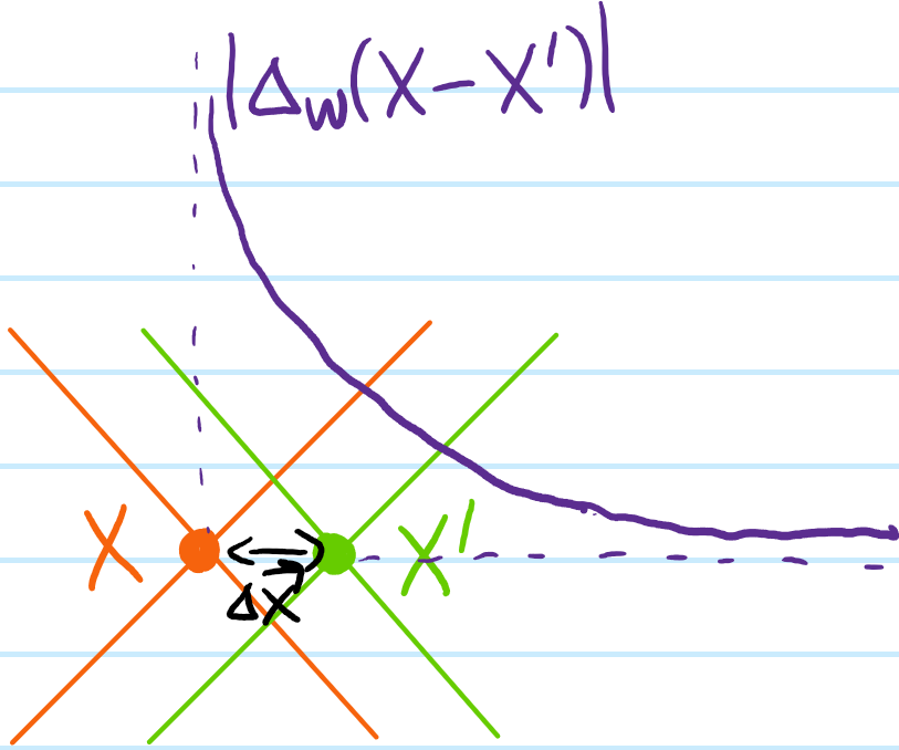
Earlier in Solution #\(11\), it was seen that for \(X=X’\), the propagator \(\Delta_W(0)=\infty\) suffered both IR and UV divergences. By contrast, if \(X\neq X’\) but instead are space-like separated events \(X-X’\approx (0,\Delta\textbf x)\), show that:
\[|\Delta_W(X-X’)|\sim e^{-k_c|\Delta\textbf x|}\]
Solution #\(14\): As usual, just plug and chug the Fourier mode expansion for \(\phi(X)\) in the Heisenberg picture. Since the ket \(|0\rangle\) is annihilated by all \(a_{\textbf k’}\) while the bra \(\langle 0|\) is annihilated by all \(a_{\textbf k}^{\dagger}\) so the only surviving combination is of the form \(a_{\textbf k}a_{\textbf k’}^{\dagger}\) which can be commuted to produce one term that annihilates as above and a delta function that kills the \(d^3\textbf k’\) integral to obtain the desired result.
For the second part, evaluate the integral in \(\textbf k\)-space spherical coordinates:
\[\Delta_W(X-X’)=\frac{\hbar c}{2(2\pi)^2}\int_0^{\infty}d|\textbf k|\frac{|\textbf k|^2}{\sqrt{|\textbf k|^2+k_c^2}}\int_0^{\pi}d\theta e^{i|\textbf k||\Delta\textbf x|\cos\theta}\sin\theta\]
\[=\frac{\hbar c}{(2\pi|\Delta\textbf x|)^2i}\int_0^{\infty}\frac{\cos x}{\sqrt{x^2+(k_c|\Delta\textbf x|)^2}}dx\]
The integral cannot be evaluated analytically, however one can apply Laplace’s saddle-point approximation to it in the limit \(a:=k_c|\Delta\textbf x|\gg 1\) of far spacelike separation:
\[\int_0^{\infty}\frac{\cos x}{\sqrt{x^2+a^2}}dx=\text{Re}\int_0^{\infty}e^{ix-\frac{1}{2}\ln(x^2+a^2)}dx\]
which is stationary when \(x^2+ix+a^2=0\Rightarrow x\approx ia\), though one has to be a bit delicate about this, in particular \(x^2+a^2=-ix=a\neq 0\). One obtains the result:
\[|\Delta_W(X-X’)|\sim |\Delta\textbf x|^{-5/2}e^{-k_c|\Delta\textbf x|}\]
in particular, even for arbitrarily spacelike separated events \(X,X’\), the quantum field “leaks” outside of the light cone in an evanescent manner. Nevertheless, this does not violate causality which only requires that \(\langle 0|[\phi_X,\phi_{X’}]|0\rangle=\Delta_W(X-X’)-\Delta_W(X’-X)=0\) vanish for spacelike separated \(|X-X’|^2<0\).
Problem #\(15\): Give \(3\) logically equivalent definitions of the Feynman propagator \(\Delta_F(X-X’)\) (useful in interacting QFTs). Show that Lorentz invariance is manifest in all \(3\) cases.
Solution #\(15\): The simplest way to think about it is that it is the time-ordered Wightman propagator:
\[\Delta_F(X-X’):=\langle 0|\mathcal T\phi_X\phi_{X’}|0\rangle:=\Delta_W(X-X’)\Theta(X^0-X’^{0})+\Delta_W(X’-X)\Theta(X’^{0}-X^0)\]
(with the convention that \(\Theta(0)=1/2\) for simultaneous events). To check that \(\Delta_F(X-X’)\) is Lorentz invariant, first note that \(\Delta_W(X-X’)\) is Lorentz invariant for any pair \(X,X’\) of events. Then, if \(|X-X’|^2>0\) are timelike-separated, their time ordering \(\Theta(X^0-X’^{0})\) is Lorentz invariant so \(\Delta_F(X-X’)\) will be Lorentz invariant. On the other hand, if \(|X-X’|^2<0\) are spacelike separated, then their time ordering will in general not be Lorentz invariant, however in that case \(\Delta_W(X-X’)=\Delta_W(X’-X)\) as established in Solution #\(14\) so regardless of how their time ordering gets shuffled, the Feynman propagator \(\Delta_F(X-X’)\) takes the same value, hence it is Lorentz invariant.
On the other hand, the Feynman propagator is also, roughly speaking, given by the off-shell integral representation (containing manifestly Lorentz invariant objects like \(d^4|K\rangle\), Minkowski inner products, etc.):
\[\Delta_F(X-X’)=\frac{i\hbar c}{(2\pi)^4}\int d^4|K\rangle\frac{e^{-i\langle K|X-X’\rangle}}{\langle K|K\rangle-k_c^2}\]
A priori, the integral is over all four-vectors \(|K\rangle\) in Minkowski spacetime which runs into trouble at the on-shell poles \(\langle K|K\rangle=k_c^2\). Thus, to be more precise, one can first write \(d^4|K\rangle=d^3\textbf kd\omega/c\) and also emphasize this by replacing \(\langle K|K\rangle-k_c^2=(\omega+\omega_{\textbf k})(\omega-\omega_{\textbf k})/c^2\), rather than integrating over the real axis \(\omega\in\textbf R\), the idea is to complexify it \(\omega\in\textbf C\) so that it hops around the on-shell poles at \(\omega=\pm\omega_{\textbf k}\) in a very specific way that enforces the time-ordering property from earlier:
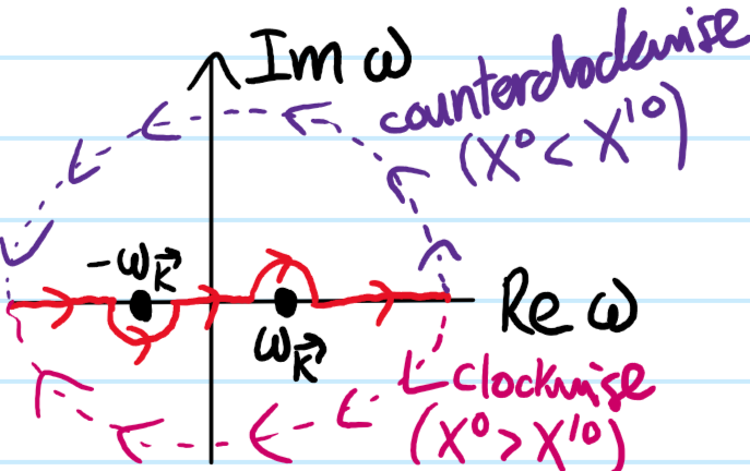
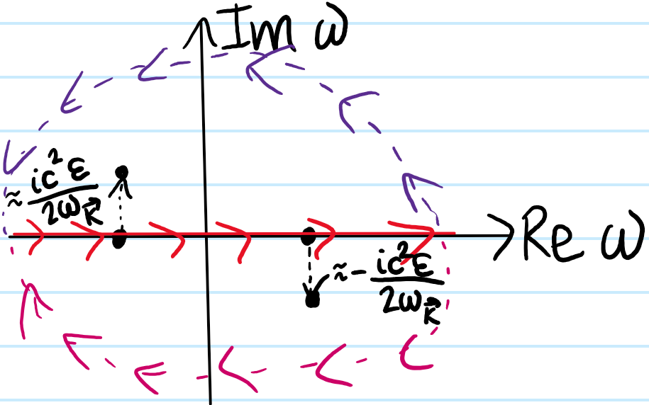
where the choice of which semicircular contour to close with is motivated by considering the time-ordering of \(X,X’\) and using Jordan’s lemma. Picking the appropriate residue in each case, one can thus verify this contour integral representation of the Feynman propagator, and indeed it is often also equivalently written without any complexification \(\omega\in\textbf R\) but instead introducing an \(i\varepsilon\)-prescription (with \(\varepsilon>0\) but infinitesimal in suitable units) to shift the poles slightly off the \(\Re\)-axis such that the pole originally at \(\omega=-\omega_{\textbf k}\) shifts slightly above the \(\Re\)-axis and vice versa for the pole at \(\omega=\omega_{\textbf k}\) to maintain the same topology as above:
\[\Delta_F(X-X’)=\frac{i\hbar c}{(2\pi)^4}\int d^4|K\rangle\frac{e^{-i\langle K|X-X’\rangle}}{\langle K|K\rangle-k_c^2+i\varepsilon}\]
(think of this as more of just a formality/notation to express a topological statement)
One last interpretation of the Feynman propagator \(\Delta_F(X-X’)\) is that, being suggestively written as a function of the argument \(X-X’\), it is essentially (irrespective of the choice of contour) a Green’s function for the Klein-Gordon operator on Minkowski spacetime:
\[(\partial^{\mu}\partial_{\mu}+k_c^2)\Delta_F(X-X’)=\frac{i\hbar c}{(2\pi)^4}\int \frac{d^4|K\rangle}{\langle K|K\rangle-k_c^2}(-\langle K|K\rangle+k_c^2)e^{-i\langle K|X-X’\rangle}\]
\[=-i\hbar c\delta^4(X-X’)\]
where note that \(\partial_{\mu}=\frac{\partial}{\partial X^{\mu}}\neq\frac{\partial}{\partial X’^{\mu}}\). This means that if one wished to solve an inhomogeneous Klein-Gordon equation with some forcing field \(f(X)\), one could just convolve \(f(X)\) with the Feynman propagator \(\Delta_F(X-X’)\) as a kernel (boundary conditions tied to a choice of contour for the Green’s function? Retarded vs. advanced Green’s functions…).