Problem: Consider an isolated atom with time-independent Hamiltonian \(H_0\). Such an atom will have many bound \(H_0\)-eigenstates, but for simplicity focus on just two such bound states (think of it as a qubit) \(|0\rangle\) and \(|1\rangle\) (called the ground state and the excited state) separated by a resonant frequency \(\omega_0=(E_1-E_0)/\hbar\). If one now proceeds to shine light on the atom of frequency \(\omega\), show that the corresponding interaction potential \(V_{/H_0}(t)\) in the interaction picture modulo \(H_0\) is given approximately by:
\[V_{/H_0}(t)\approx \frac{\hbar\Omega}{2}(e^{-i\delta t}\sigma_++h.c.)\]
where the detuning \(\delta:=\omega-\omega_0\), and state all assumptions.
Solution: The assumptions are:
- (Semiclassical approximation) The atom is treated “quantumly” but the light is treated classically.
- (\(\alpha\times\)Stark \(=\) Zeeman) Within the semiclassical approximation, the effect of the \(\textbf B\)-field is ignored compared to the \(\textbf E\)-field.
- (Dipole approximation) The electric field is approximately spatially independent \(\textbf E(t)=\textbf E_0\cos(\omega t)\) (by evaluating it at the atom’s position).
- (Two-level system) Assume no other \(H_0\)-eigenstates are relevant, i.e. \(|0\rangle\langle 0|+|1\rangle\langle 1|\approx 1\).
- (\([H_0,\Pi]=0\)) The ground state \(|0\rangle\) and the excited state \(|1\rangle\) are both \(\Pi\)-eigenstates with opposite parity eigenvalues \(\pm 1\).
- (Rotating wave approximation) The detuning is small, i.e. \(|\delta|\ll\omega+\omega_0\) (notice this is compatible with assumption #\(4\)).
- (Monochromatic) The light is assumed to be of a single frequency \(\omega\) with zero spectral width.
Then the interaction potential in the Schrodinger picture is:
\[V(t)=-\boldsymbol{\pi}\cdot\textbf E(t)=\hbar\Omega\cos\omega t\sigma_x\]
where the matrix elements are in the obvious Hilbert space \(\text{span}_{\textbf C}|0\rangle,|1\rangle\) and the diagonal entries vanish by the parity assumption. Here, \(\Omega\) is the Rabi frequency and defined to capture those non-vanishing off-diagonal matrix elements (both gauge-fixed to be real):
\[\hbar\Omega:=\langle 1|-\boldsymbol{\pi}\cdot\textbf E_0|0\rangle=\langle 0|-\boldsymbol{\pi}\cdot\textbf E_0|1\rangle\]
(intuition: \(\Omega\) simultaneously contains information about how “bright” the light is and also how strongly this particular E\(1\) perturbation couples \(|0\rangle\) and \(|1\rangle\)). In the interaction picture modulo \(H_0\):
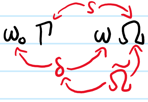
\[V_{/H_0}(t)=e^{iH_0t/\hbar}V(t)e^{-iH_0t/\hbar}\]
\[=\hbar\Omega\cos\omega t\text{diag}(e^{iE_0t/\hbar},e^{iE_1t/\hbar})\sigma_x\text{diag}(e^{-iE_0t/\hbar},e^{-iE_1t/\hbar})\]
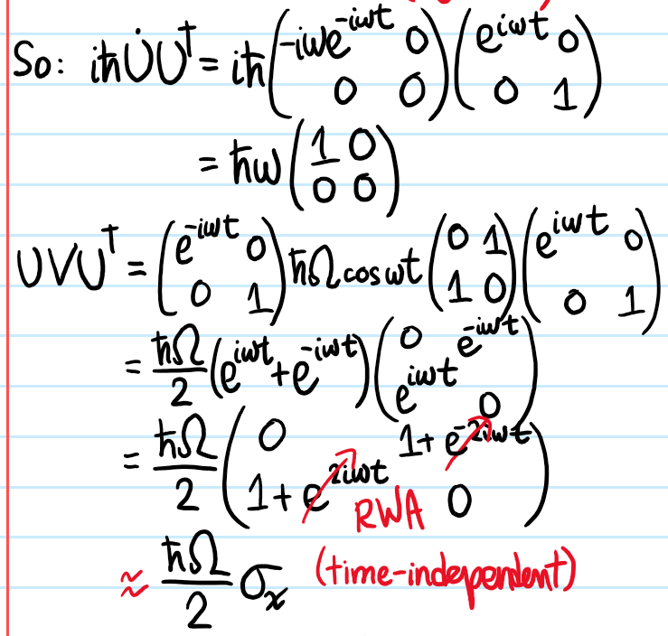
\[=\hbar\Omega\cos\omega t\begin{pmatrix}0&e^{-i\omega_0 t}\\e^{i\omega_0 t}&0\end{pmatrix}\]
\[\approx\frac{\hbar\Omega}{2}\begin{pmatrix}0&e^{i\delta t}\\e^{-i\delta t}&0\end{pmatrix}\]
where one has written \(\cos \omega t=(e^{i\omega t}+e^{-i\omega t})/2\) to make the “lock-in detection” explicit and then low-pass filtered with RWA. In particular, seeing the factor of \(1/2\) in front is a smoking gun for RWA. This then matches the claimed result with \(\sigma_+:=|1\rangle\langle 0|=\begin{pmatrix}0&0\\1&0\end{pmatrix}\) and \(\sigma_{\pm}^{\dagger}=\sigma_{\mp}\).
Problem: Having found \(V_{/H_0}(t)\), show that \(|\psi_{/H_0}(t)\rangle\) undergoes Rabi oscillations at the generalized Rabi frequency \(\tilde{\Omega}:=\sqrt{\Omega^2+\delta^2}\).
If one expands out the interaction picture state \(|\psi_I(t)\rangle=\langle 0|\psi_I(t)\rangle|0\rangle+\langle 1|\psi_I(t)\rangle|1\rangle\) in the subspace as well, then one obtains a non-autonomous linear dynamical system with \(2\pi/\delta\)-periodic Floquet forcing:
\[\begin{pmatrix}\dot{\langle 0|\psi_I\rangle}\\\dot{\langle 1|\psi_I\rangle}\end{pmatrix}=\frac{\Omega}{2i}\begin{pmatrix}0&e^{i\delta t}\\e^{-i\delta t}&0\end{pmatrix}\begin{pmatrix}\langle 0|\psi_I\rangle\\\langle 1|\psi_I\rangle\end{pmatrix}\]
Nevertheless, it turns out to be very easy in this case to decouple the time evolutions of the projections \(\langle 0|\psi_I\rangle\) and \(\langle 1|\psi_I\rangle\) from each other into two undriven, damped harmonic oscillators (even though ironically the atom is being driven with light at \(\omega_{\text{ext}}=\omega_{01}+\delta\)):
\[\ddot{\langle 0|\psi_I\rangle}-i\delta\dot{\langle 0|\psi_I\rangle}+\frac{\Omega^2}{4}\langle 0|\psi_I\rangle=0\]
\[\ddot{\langle 1|\psi_I\rangle}+i\delta\dot{\langle 1|\psi_I\rangle}+\frac{\Omega^2}{4}\langle 1|\psi_I\rangle=0\]
Assuming the initial condition \(|\psi_I(0)\rangle=|0\rangle\) that the atom starts at time \(t=0\) in the ground state \(|0\rangle\), the solutions are:
\[\langle 0|\psi_I(t)\rangle=e^{i\delta t/2}\left(\cos\frac{\tilde{\Omega}}{2}t-\frac{i\delta}{\tilde{\Omega}}\sin\frac{\tilde{\Omega}}{2}t\right)\]
and more intuitively:
\[\langle 1|\psi_I(t)\rangle=-ie^{-i\delta t/2}\frac{\Omega}{\tilde{\Omega}}\sin\frac{\tilde{\Omega}}{2}t\]
where \(\tilde{\Omega}:=\sqrt{\Omega^2+\delta^2}\) is called the generalized Rabi frequency. Being a harmonic oscillator, it makes sense that the atom’s interaction picture state \(|\psi_I(t)\rangle\) roughly speaking “oscillates” between the ground state \(|0\rangle\) and the excited state \(|1\rangle\), called Rabi oscillations, but these oscillations are not actually damped because the “damping coefficient” \(\pm i\delta\) was imaginary. Note that although all of the above discussion has focused on Rabi oscillations in the context of electric dipole transitions, there are also times when the magnetic field \(\textbf B_{\text{ext}}\) rather than the electric field \(\textbf E_{\text{ext}}\) dominates the physics (e.g. fine structure or hyperfine structure transitions) in which case there would also be Rabi oscillations in the context of magnetic dipole transitions.
Rabi oscillations are more intuitive when expressed in terms of the probabilities prescribed by the Born rule. In this case, one has (dropping the \(I\)-subscript because it no longer matters):
\[|\langle 0|\psi(t)\rangle|^2=1-|\langle 1|\psi(t)\rangle|^2\]
\[|\langle 1|\psi(t)\rangle|^2=\frac{\Omega^2}{\tilde{\Omega}^2}\sin^2\frac{\tilde{\Omega}}{2}t\]
where remember that \(\sin^2\frac{\tilde{\Omega}}{2}t=\frac{1}{2}(1-\cos\tilde{\Omega}t)\) oscillates at the generalized Rabi frequency \(\tilde{\Omega}\) and not \(\tilde{\Omega}/2\). In particular, these Rabi “probability oscillations” are most pronounced when the light is resonant with the atom, i.e. \(\delta=0\). In this case, \(\tilde{\Omega}=\Omega\) and one has:
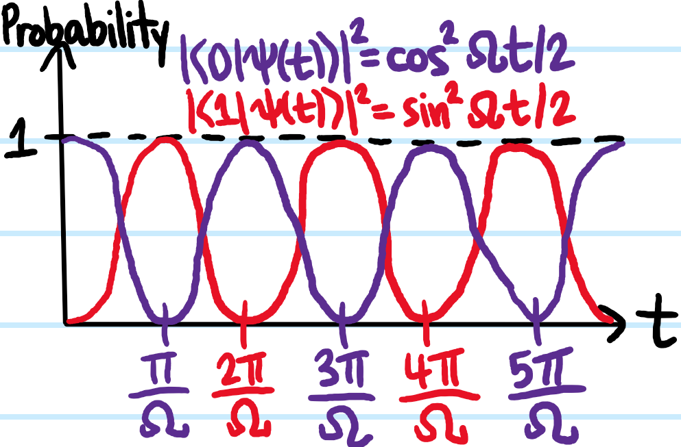
Such \(\delta=0\) resonant Rabi oscillations also provide a way to experimentally prepare various qubit states in the lab simply by controlling the driving time \(\Omega t\) for which one applies the light. For instance, if one applies a \(\pi\)-pulse so that \(\Omega t=\pi\), then in theory one is guaranteed to excite the atom \(|0\rangle\mapsto -i|1\rangle\equiv|1\rangle\). Alternatively, if one applies an \(\Omega t=\pi/2\)-pulse, then this yields the “circularly polarized” state \(|0\rangle\mapsto (|0\rangle-i|1\rangle)/\sqrt{2}\).
More generally when the detuning \(\delta\neq 0\) is off-resonance, the maximum probability of an electric dipole transition \(|0\rangle\to|1\rangle\) from the ground state to the excited state that one can achieve is \(\Omega^2/\tilde{\Omega}^2\), although in the limit as \(\Omega\to\infty\) (e.g. cranking up the laser), this ratio does approach \(1\).
As with any qubit system, one can visualize the dynamics of Rabi oscillations on the Bloch sphere. Although here the ket \(|\psi_I(t)\rangle\) is tautologically a pure state, one can nevertheless work with its interaction picture density operator \(\rho_I(t)=|\psi_I(t)\rangle\langle\psi_I(t)|\). However, despite one’s first instinct being to work with \(\rho_I\) in the \(H\)-eigenbasis of the ground state \(|0\rangle\) and excited state \(|1\rangle\), it turns out to be more convenient to first boost unitarily into a “steady-state picture”. Specifically, if one instead works with the “steady-state basis” \(|\tilde 0\rangle:=e^{i\delta t/2}|0\rangle\) and similarly \(|\tilde 1\rangle:=e^{-i\delta t/2}|1\rangle\), along with the bras \(\langle\tilde 0|=e^{-i\delta t/2}\langle 0|\) and \(\langle\tilde 1|=e^{i\delta t/2}\langle 1|\), then starting from the earlier Schrodinger equation in the rotating wave approximation:
\[\begin{pmatrix}\dot{\langle 0|\psi_I\rangle}\\\dot{\langle 1|\psi_I\rangle}\end{pmatrix}=\frac{\Omega}{2i}\begin{pmatrix}0&e^{i\delta t}\\e^{-i\delta t}&0\end{pmatrix}\begin{pmatrix}\langle 0|\psi_I\rangle\\\langle 1|\psi_I\rangle\end{pmatrix}\]
the benefit of this change of basis is that the new “steady-state Hamiltonian” \(H_{\infty}\):
\[H_{\infty}=\frac{\hbar}{2}\begin{pmatrix}\delta&\Omega\\\Omega&-\delta\end{pmatrix}=\frac{\hbar}{2}\tilde{\boldsymbol{\Omega}}\cdot\boldsymbol{\sigma}\]
for which
\[\begin{pmatrix}\dot{\langle\tilde 0|\psi_I\rangle}\\\dot{\langle \tilde 1|\psi_I\rangle}\end{pmatrix}=\frac{1}{2i}\begin{pmatrix}\delta&\Omega\\\Omega&-\delta\end{pmatrix}\begin{pmatrix}\langle\tilde 0|\psi_I\rangle\\\langle \tilde 1|\psi_I\rangle\end{pmatrix}\]
is now time-independent at the expense of gaining back the diagonal matrix elements, where the generalized Rabi vector is given by \(\tilde{\boldsymbol{\Omega}}:=(\Omega,0,\delta)\) and has magnitude equal to the generalized Rabi frequency \(|\tilde{\boldsymbol{\Omega}}|=\sqrt{\Omega^2+\delta^2}\).
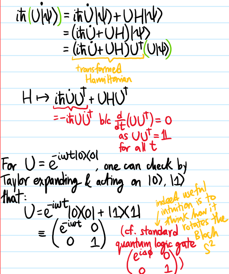
Problem: Show that this result can also be obtained by transforming to an alternative picture (rather than the standard interaction picture mod \(H_0\)):
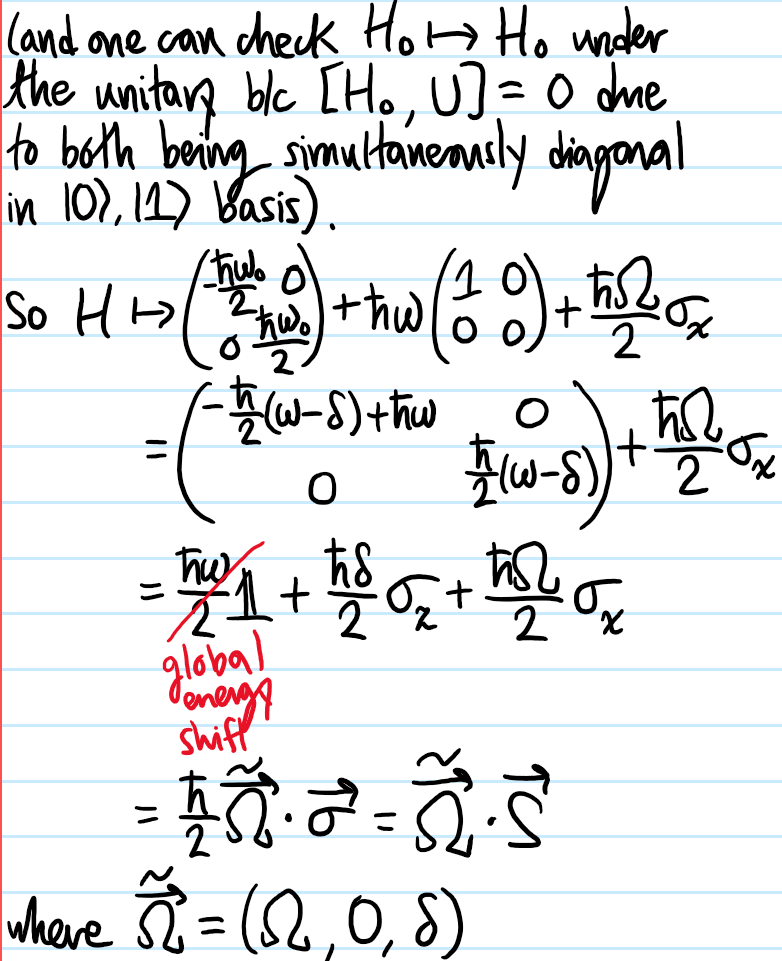
- Split \(H_0=E_0|0\rangle\langle 0|+E_1|1\rangle\langle 1|\) into symmetric and antisymmetric parts:
\[H_0=\frac{E_0+E_1}{2}1+\frac{\hbar\omega_0}{2}\left(|1\rangle\langle 1|-|0\rangle\langle 0|\right)\]
And since the symmetric part is isotropic, one can safely discard it and keep only the antisymmetric part.
2. Starting from the Schrodinger picture, transform into a picture defined by the unitary \(U(t):=e^{-i\omega t|0\rangle\langle 0|}\).
3. Apply the rotating wave approximation.
Solution: The first part is straightforward. Then:
In this steady-state basis \(|\tilde 0\rangle,|\tilde 1\rangle\), the density matrix \([\rho_I(t)]_{|\tilde 0\rangle,|\tilde 1\rangle}^{|\tilde 0\rangle,|\tilde 1\rangle}=\frac{1}{2}(1+\tilde{\textbf b}\cdot\boldsymbol{\sigma})\) can be replaced by the conceptually simpler Bloch vector \(\tilde{\textbf b}\in\textbf R^3\) of the qubit whose components \(\tilde{\textbf b}=(\tilde b_1,\tilde b_2,b_3)\) relate back to the matrix elements of the density operator \(\rho_I\) via:
\[\tilde b_1=\tilde{\rho}_{01}+\tilde{\rho}_{10}\]
\[\tilde b_2=i(\tilde{\rho}_{01}-\tilde{\rho}_{10})\]
\[b_3=\rho_{00}-\rho_{11}\]
where the populations \(\tilde{\rho}_{00}=\rho_{00},\tilde{\rho}_{11}=\rho_{11}\) are unaffected by the boost (relative to if the matrix elements of \(\rho_I\) were expressed in the \(|0\rangle,|1\rangle\) basis) and the coherences \(\tilde{\rho}_{01}=e^{-i\delta t}\rho_{01},\tilde{\rho}_{10}=e^{i\delta t}\rho_{10}\) are affected:
\[[\rho_I(t)]_{|\tilde 0\rangle,|\tilde 1\rangle}^{|\tilde 0\rangle,|\tilde 1\rangle}=\begin{pmatrix}\rho_{00}&\tilde{\rho}_{01}\\ \tilde{\rho}_{10}&\rho_{11}\end{pmatrix}=\begin{pmatrix}\langle 0|\rho|0\rangle & \langle\tilde 0|\rho|\tilde 1\rangle \\ \langle\tilde 1|\rho|\tilde 0\rangle & \langle 1|\rho|1\rangle\end{pmatrix}=\begin{pmatrix}|\langle 0|\psi_I\rangle|^2 & \langle \tilde 0|\psi_I\rangle\langle\psi_I|\tilde 1\rangle \\ \langle\tilde 1|\psi_I\rangle\langle\psi_I|\tilde 0\rangle & |\langle 1|\psi_I\rangle|^2\end{pmatrix}\]
From Liouville’s equation \(i\hbar\dot{\rho}_I=[H_{\infty},\rho_I]\) and the standard identity of Pauli matrices \([\tilde{\boldsymbol{\Omega}}\cdot\boldsymbol{\sigma},\tilde{\textbf b}\cdot\boldsymbol{\sigma}]=2i(\tilde{\boldsymbol{\Omega}}\times\tilde{\textbf b})\cdot\boldsymbol{\sigma}\), one immediately obtains the precession of the Bloch vector \(\tilde{\textbf b}\) around the generalized Rabi vector \(\tilde{\boldsymbol{\Omega}}\) at the generalized Rabi frequency:
\[\dot{\tilde{\textbf b}}=\tilde{\boldsymbol{\Omega}}\times\tilde{\textbf b}\]
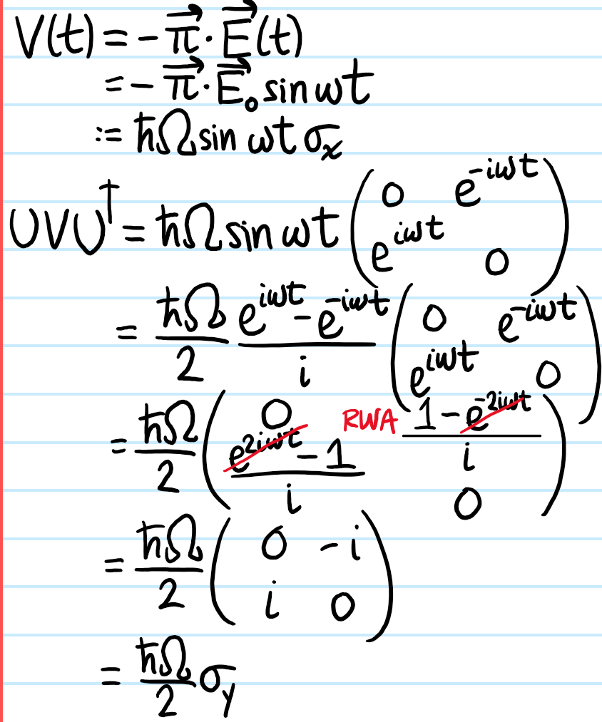
For large detunings \(\delta\), the Bloch vector \(\tilde{\textbf b}\) precesses faster (i.e. one gets faster Rabi oscillations) though at the expense of the maximum excited population \(\text{max}(\rho_{11})=\Omega^2/\tilde{\Omega}^2\) achievable (as already mentioned before). Note also that the generalized Rabi vector \(\tilde{\boldsymbol{\Omega}}\) does depend on when one starts the clock; for instance if \(\textbf E_{\text{ext}}(\textbf x,t)=\textbf E_0\sin(\textbf k_{\text{ext}}\cdot\textbf x-\omega_{\text{ext}}t)\) instead of \(\cos\), then in this case \(\tilde{\boldsymbol{\Omega}}=(0,\Omega,\delta)\) instead, etc.
Optical Bloch Equations
From the stimulated absorption and emission interactions of the atom with the external optical field, Rabi oscillations were seen to emerge. However, Einstein’s statistical argument showed that in addition to stimulated absorption/emission, there is also spontaneous emission. How does this affect the physics? Although a rigorous treatment requires quantizing the EM field, phenomenologically one can simply include a decay term (in the spirit of Einstein) of the form \(-\Gamma\rho_{11}\) (where \(\Gamma=A_{10}\) in the Einstein model) to the rate equation for the excited state population \(\dot{\rho}_{11}=\frac{\Omega}{2}\tilde{b}_2-\Gamma\rho_{11}\). At low laser intensities, \(\Gamma\sim 2\pi\times 10\text{ MHz}\) will in fact typically be greater than the Rabi frequency \(\Omega\), making spontaneous decay an important mechanism by which otherwise coherent Rabi oscillations decohere over time. Although it is immediate that \(\dot b_3=-\Omega\tilde b_2-\Gamma(b_3-1)\), what is not so clear is how \(\tilde b_1,\tilde b_2\) are affected by the spontaneous decay \(\Gamma\neq 0\). By analogy with a classical damped electric dipole, it turns out one can phenomenologically obtain the optical Bloch equations:
\[\dot{\tilde b}_1=\delta\tilde b_2-\frac{\Gamma}{2}\tilde b_1\]
\[\dot{\tilde b}_2=-\delta\tilde b_1+\Omega b_3-\frac{\Gamma}{2}\tilde b_2\]
\[\dot b_3=-\Omega\tilde b_2-\Gamma(b_3-1)\]
Unlike the earlier precession \(\dot{\tilde{\textbf b}}=\tilde{\boldsymbol{\Omega}}\times\tilde{\textbf b}\) in the absence \(\Gamma=0\) of spontaneous emissions, now, in the steady state limit \(t\gg 1/\Gamma\) of long driving times where \(\dot{\tilde b}_1=\dot{\tilde b}_2=\dot b_3=0\), the Bloch vector eventually settles onto:
\[\tilde{\textbf b}_{\infty}=\frac{1}{\delta^2+\Omega^2/2+\Gamma^2/4}\begin{pmatrix}\Omega\delta\\\Omega\Gamma/2\\\delta^2+\Gamma^2/4\end{pmatrix}\]
In particular, an immediate important corollary is:
\[\rho_{11}=\frac{\Omega^2/4}{\delta^2+\Omega^2/2+\Gamma^2/4}\]
along with the strongly driven limit \(\rho_{11}\to 1/2\) of the excited state population as \(\Omega\to\infty\). Equivalently, in terms of the spontaneous decay rate \(\gamma:=\Gamma\rho_{11}\), one has:
\[\gamma=\frac{\Gamma}{2}\frac{s}{1+s+(2\delta/\Gamma)^2}\]
with \(s=2(\Omega/\Gamma)^2:=I/I_{\text{sat}}\) the normalized intensity. Thus, one’s intuition would suggest that simply cranking up the laser intensity \(s\to\infty\) should excite all atoms into the excited state \(|1\rangle\), the spontaneous decay rate \(\gamma\to\Gamma/2\) prevents one from achieving this.