
Problem #\(1\): Consider a simplistic classical model of an atom as a positively charged nucleus \(Q>0\) surrounded by a spherical, uniformly dense electron cloud \(-Q<0\) of radius \(a\). If this atom is subjected to a DC external electric field \(\textbf E_{\text{ext}}\), show that the induced dipole \(\textbf p_{\text{ind}}\) developed by the atom is given by \(\textbf p_{\text{ind}}=\alpha\textbf E_{\text{ext}}\) where the atomic polarizability is given by \(\alpha=4\pi\varepsilon_0 a^3>0\). Neglect any higher-order multipole moments of the electron cloud (i.e. assume it maintains a spherical shape when perturbed by \(\textbf E_{\text{ext}}\)).
Solution #\(1\): By Gauss’s law for electric fields, the internal electrostatic field \(\textbf E_{\text{int}}(\textbf x)\) due to just the electron cloud must rise linearly in magnitude to match the Coulomb field at \(|\textbf x|=a\), thus \(\textbf E_{\text{int}}(|\textbf x|=a)=-Q/4\pi\varepsilon_0 a^2\hat{\textbf x}\), hence \(\textbf E_{\text{int}}(\textbf x)=-Q|\textbf x|/4\pi\varepsilon_0 a^3\hat{\textbf x}\) for \(|\textbf x|\leq a\). When the external electric field \(\textbf E_{\text{ext}}\) is applied, this will induce a displacement of the nucleus to a new equilibrium \(\textbf x=\textbf 0\mapsto\textbf x=\Delta\textbf x_{\text{ind}}\) relative to the center of the electron cloud, at which location force balance requires:
\[\textbf E_{\text{int}}(\Delta\textbf x_{\text{ind}})+\textbf E_{\text{ext}}=\textbf 0\]
Noting that the induced dipole is \(\textbf p_{\text{ind}}=Q\Delta\textbf x_{\text{ind}}\), the claim follows.
Problem #\(2\): Explain what it means for a dielectric to be linear and explain under what circumstances can most dielectrics be modelled as linear.
Solution #\(2\): A dielectric is said to be linear iff, when subjected to an external (not necessarily uniform or DC!) electric field \(\textbf E_{\text{ext}}\), the induced polarization \(\textbf P_{\text{ind}}\) is linear in \(\textbf E_{\text{ext}}\) in the sense that there exists an electric susceptibility \(\chi_e\) such that:
\[\textbf P_{\text{ind}}=\varepsilon_0\chi_e\textbf E_{\text{ext}}\]
By definition, \(\textbf P_{\text{ind}}:=n_{\textbf p_{\text{ind}}}\textbf p_{\text{ind}}\) is the number density \(n_{\textbf p_{\text{ind}}}\) of induced electric dipoles \(\textbf p_{\text{ind}}\). If \(\textbf E_{\text{ext}}\) is DC as in Problem #\(1\), then in that case \(\chi_e>0\) is real and given by \(\chi_e=4\pi n_{\textbf p_{\text{ind}}}a^3\). In general, the assumption of linearity is only a good approximation provided \(|\textbf E_{\text{ext}}|\) is not too strong.
Problem #\(3\): Explain what the concept of bound charge is and show that the surface bound charge density \(\sigma_b\) and the volume bound charge density \(\rho_b\) are related to the polarization \(\textbf P\) via:
\[\sigma_b=\hat{\textbf n}\cdot\textbf P\]
\[\rho_b=-\frac{\partial}{\partial\textbf x}\cdot\textbf P\]
Comment on the case where \(\textbf P\) is uniform within a material.
Solution #\(3\): Whenever, for any reason whatsoever, there is a polarization \(\textbf P\neq\textbf 0\) (often when an \(\textbf E_{\text{ext}}\) is applied such as in Problems #\(1\) and #\(2\), though see ferroelectrics), then there must necessarily be a build-up of electric charge somewhere in a material volume \(V\) (or on its surface \(\partial V\)); any such charge is called bound charge. This is because the electrostatic potential \(\phi\) induced by this \(\textbf P\) would be given by:
\[\phi(\textbf x)=\frac{1}{4\pi\varepsilon_0}\iiint_{\textbf x’\in V}\frac{\textbf P(\textbf x’)\cdot(\textbf x-\textbf x’)}{|\textbf x-\textbf x’|^3}d^3\textbf x’\]
But noting that (e.g. in spherical coordinates) \(\frac{\partial}{\partial\textbf x’}\frac{1}{|\textbf x-\textbf x’|}=\frac{\textbf x-\textbf x’}{|\textbf x-\textbf x’|^3}\), an integration by parts shows that:
\[\phi(\textbf x)=\frac{1}{4\pi\varepsilon_0}\iint_{\textbf x’\in\partial V}\frac{\sigma_b(\textbf x’)}{|\textbf x-\textbf x’|}d^2\textbf x’+\frac{1}{4\pi\varepsilon_0}\iiint_{\textbf x’\in V}\frac{\rho_b(\textbf x’)}{|\textbf x-\textbf x’|}d^3\textbf x’\]
(note that right now both of these are only electrostatic results because they arise by comparison to Coulomb’s law). When \(\textbf P\) is uniformly polarized, then bound charge does not clump up anywhere inside the material \(\rho_b=0\), but only on its surface \(\sigma_b\neq 0\).
Problem #\(4\): Explain what the concept of free charge is, and show that for a linear dielectric sphere of radius \(R\) with a lump of charge \(Q_f\) deposited at its center, the surface bound charge density is \(\sigma_b=\frac{\chi_e Q_f}{4\pi R^2(1+\chi_e)}\). What is the corresponding discontinuity \(\Delta\textbf E\) in the \(\textbf E\)-field across the surface of the linear dielectric sphere?
Solution #\(4\): Free charge is any charge that has clumped somewhere in a material, but that is not due to polarization \(\textbf P\), i.e. it is not bound charge. Essentially, it is a wastebasket for non-bound charge so that \(\rho=\rho_f+\rho_b\). Defining the displacement field as \(\textbf D:=\varepsilon_0\textbf E+\textbf P\) so that \(\frac{\partial}{\partial\textbf x}\cdot\textbf D=\rho_f\), it follows that for the free charge distribution \(\rho_f(\textbf x)=Q_f\delta^3(\textbf x)\), one has (everywhere in space \(\textbf x\in\textbf R^3-\{\textbf 0\}\), not just inside the dielectric sphere!):
\[\textbf D(\textbf x)=\frac{Q_f}{4\pi|\textbf x|^2}\hat{\textbf x}\]
Outside the dielectric sphere \(|\textbf x|\geq R\) where \(\textbf P=\textbf 0\), this reproduces the usual electric field \(\textbf E(\textbf x)=Q_f/4\pi\varepsilon_0|\textbf x|^2\hat{\textbf x}\). Meanwhile, for \(|\textbf x|\leq R\), the assumption of dielectric linearity allows one to write \(\textbf D=\varepsilon\textbf E\) with the permittivity \(\varepsilon=\varepsilon_0(1+\chi_e)\), yielding an internal electric field \(\textbf E(\textbf x)=Q_f/4\pi\varepsilon|\textbf x|^2\hat{\textbf x}\) screened by bound charge, and a corresponding induced polarization:
\[\textbf P(\textbf x)=\frac{\chi_e Q_f}{4\pi(1+\chi_e)|\textbf x|^2}\hat{\textbf x}\]
The claim then follows from \(\sigma_b=\hat{\textbf x}\cdot\textbf P(|\textbf x|=R)\). Alternatively, the bound charge \(\rho_b(\textbf x)=Q_b\delta^3(\textbf x)\) polarized towards the origin is clearly (using \(\rho_b=-\partial/\partial\textbf x\cdot\textbf P\) and the divergence theorem) \(Q_b=-\chi_eQ_f/(1+\chi_e)\) so that the net charge at the origin is \(Q_f+Q_b=Q_f/(1+\chi_e)\), consistent with the form of the \(\textbf E\)-field inside the linear dielectric sphere. But since the sphere as a whole should only contain the central free charge \(Q_f\), this requires it to have surface charge \(-Q_b\) from which \(\sigma_b=-Q_b/4\pi R^2\) leads to the same answer.
Although the \(\textbf D\)-field is continuous \(\Delta\textbf D=\textbf 0\) across the sphere surface (from \(\frac{\partial}{\partial\textbf x}\cdot\textbf D=\rho_f\) and a Gaussian pillbox, this is seen to be due to the lack of free surface charges \(\sigma_f=0\)), the \(\textbf E\)-field discontinuity is \(\Delta\textbf E=\sigma_b/\varepsilon_0\).
Problem #\(5\): Derive the analog of Problem #\(3\) for magnetostatics.
Solution #\(5\): Everything is completely analogous, in particular the analog of \(\phi\) is \(\textbf A\):
\[\textbf A(\textbf x)=\frac{\mu_0}{4\pi}\iiint_{\textbf x’\in V}\frac{\textbf M(\textbf x’)\times(\textbf x-\textbf x’)}{|\textbf x-\textbf x’|^3}d^3\textbf x’\]
Applying the same identity and tricks as in Solution #\(3\):
\[\textbf A(\textbf x)=\frac{\mu_0}{4\pi}\iint_{\textbf x’\in\partial V}\frac{\textbf K_b(\textbf x’)}{|\textbf x-\textbf x’|}d^2\textbf x’+\frac{\mu_0}{4\pi}\iiint_{\textbf x’\in V}\frac{\textbf J_b(\textbf x’)}{|\textbf x-\textbf x’|}d^3\textbf x’\]
where the bound surface current is \(\textbf K_b=\textbf M\times\hat{\textbf n}\) and the bound current is \(\textbf J_b=\frac{\partial}{\partial\textbf x}\times\textbf M\) (note that right now both of these are only magnetostatic results because they arise by comparison to the Biot-Savart law).
Problem #\(6\): Unfortunately there is no simple classical analog of Problem #\(1\) that can be used to rationalize why it is the case that many materials are linear not just as dielectrics, but also as diamagnets/paramagnets (quantum mechanics is needed!). So for now, taking as an experimental fact that \(\textbf M_{\text{ind}}=\chi_m\textbf H_{\text{ext}}\) for some magnetic susceptibility \(\chi_m\in\textbf R\), explain why \(\mu=\mu_0(1+\chi_m)\) (cf. \(\varepsilon=\varepsilon_0(1+\chi_e)\)).
Solution #\(6\): Most of the time when one thinks of “current”, one is thinking of free current \(\textbf J_f\) which contributes to the magnetic field \(\textbf B\) on top of any bound current \(\textbf J_b\) due to magnetization \(\textbf M\neq\textbf 0\). Ampere’s law of magnetostatics asserts that:
\[\frac{\partial}{\partial\textbf x}\times\textbf B=\mu_0(\textbf J_f+\textbf J_b)\]
So this motivates the definition of the magnetizing field \(\textbf H:=\textbf B/\mu_0-\textbf M\) so that \(\partial/\partial\textbf x\times\textbf H=\textbf J_f\). That being said, analogous to how \(\textbf D=\varepsilon\textbf E\) in linear dielectrics, one would also like \(\textbf H=\textbf B/\mu\) in these “linear diamagnets/paramagnets”. The claim follows.
Problem #\(7\): Explain what changes of the electrostatic/magnetostatic results above when the fields are taken to depend on time \(t\).
Solution #\(7\): Just as Maxwell’s displacement current contribution to Ampere’s original magnetostatic law came about by enforcing local charge conservation, here the idea will be to enforce local bound charge conservation, with local free charge conservation therefore coming as a corollary. As usual, this means stipulating the continuity equation:
\[\frac{\partial\rho_b}{\partial t}+\frac{\partial}{\partial\textbf x}\cdot\textbf J_b=0\]
The earlier magnetostatic result \(\textbf J_b=\partial/\partial\textbf x\times\textbf M\) is clearly not compatible with this if \(\dot{\rho}_b\neq 0\) is changing, and therefore, because \(\rho_b=-\partial/\partial\textbf x\cdot\textbf P\), needs to be corrected to:
\[\textbf J_b=\frac{\partial}{\partial\textbf x}\times\textbf M+\frac{\partial\textbf P}{\partial t}\]
Problem #\(8\): Write down Maxwell’s equations in materials. Comment on the case \(\rho_f=0\) and \(\textbf J_f=\textbf 0\).
Solution #\(8\):
\[\frac{\partial}{\partial\textbf x}\cdot\textbf D=\rho_f\]
\[\frac{\partial}{\partial\textbf x}\cdot\textbf B=0\]
\[\frac{\partial}{\partial\textbf x}\times\textbf E=-\frac{\partial\textbf B}{\partial t}\]
\[\frac{\partial}{\partial\textbf x}\times\textbf H=\textbf J_f+\frac{\partial\textbf D}{\partial t}\]
These should always be viewed with in conjunction with a pair of constitutive relations, usually just the linear approximations \(\textbf D=\varepsilon\textbf E\) and \(\textbf H=\textbf B/\mu\). In dielectrics where \(\rho_f=0\) and \(\textbf J_f=\textbf 0\), Maxwell’s equations look like the usual ones in vacuum but with \(\varepsilon_0\mapsto\varepsilon\) and \(\mu_0\mapsto\mu\) (assuming the dielectric is linear). Light waves can therefore propagate in linear dielectrics just as they would in vacuum, except at a slower speed \(v=(\mu\varepsilon)^{-1/2}<c\).
Problem #\(9\): Using the results of Solution #\(8\), derive the \(4\) electromagnetic interface conditions (hint: each of the \(4\) macroscopic Maxwell equations will provide one).
Solution #\(9\): “Use pillboxes for the divs and closed loops for the curls”:
\[\Delta\textbf D\cdot\hat{\textbf n}=\sigma_f\]
\[\Delta\textbf B\cdot\hat{\textbf n}=0\]
\[\hat{\textbf n}\times\Delta\textbf E=\textbf 0\]
\[\hat{\textbf n}\times\Delta\textbf H=\textbf K_f\]
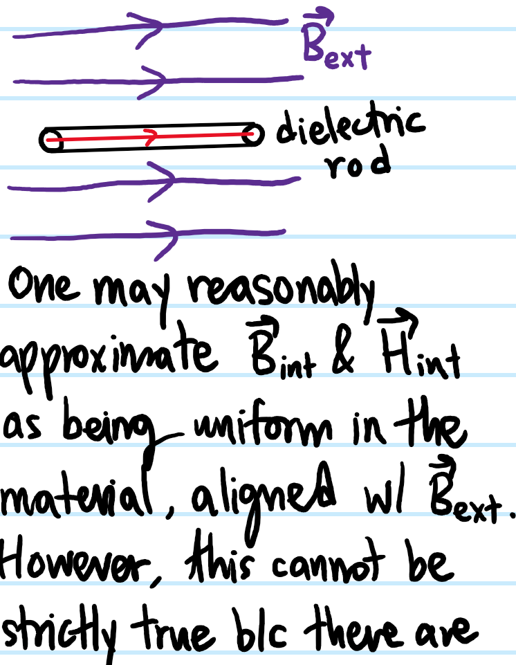
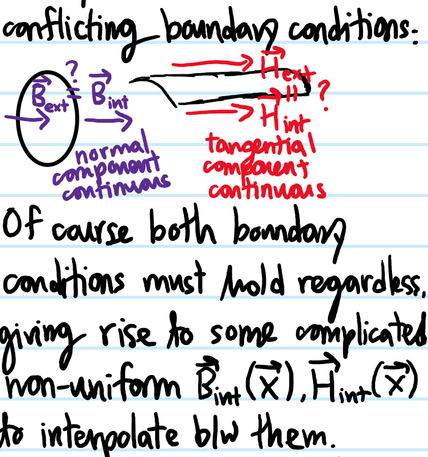
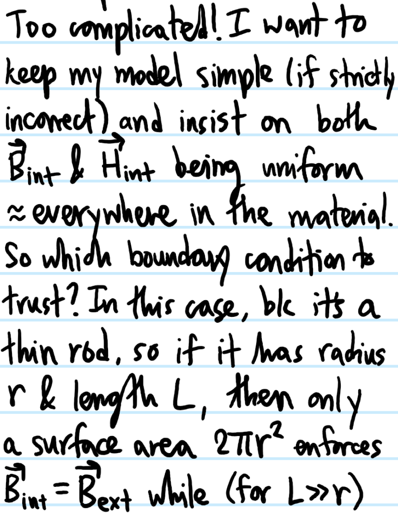
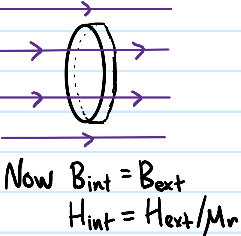
Problem: Consider placing a thin rod aligned with an external magnetic field \(\textbf B_{\text{ext}}\). What is the internal magnetic field \(\textbf B_{\text{int}}\) and magnetizing field \(\textbf H_{\text{int}}\)?
Solution:
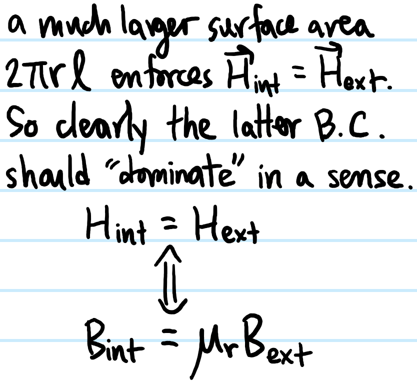
Problem: Repeat the above problem but for a thin slab.
Solution: Following the discussion above, the dominant boundary condition is the normal continuity of the \(\textbf B\)-field:
Problem #\(10\): Derive the law of reflection and Snell’s law.
Solution #\(10\): Applying phase-matching at the \(z=0\) interface (otherwise there could be no hope of satisfying the electromagnetic interface conditions), one concludes that the frequency is solely a property of the incident source \(\omega=\omega’=\omega^{\prime\prime}\), reflecting conservation of photon energy, and that the projections \(k\sin\theta=k’\sin\theta’=k^{\prime\prime}\sin\theta^{\prime\prime}\) of the wavevectors \(\textbf k,\textbf k’\) and \(\textbf k^{\prime\prime}\) onto the \(xy\)-plane \(z=0\) are also equal, reflecting conservation of photon momentum along that direction. The law of reflection then follows simply because the reflected ray is in the same dielectric \(n^{\prime\prime}=n\) as the incident ray, while Snell’s law \(n\sin\theta=n’\sin\theta’\) follows because the refracted ray is now in a different dielectric \(n’\neq n\) with different dispersion relation.
(aside: provided the media actually support wave propagation and that all indices of refraction are defined via the phase velocity so that \(n,n’\) could be less than \(1\), then both the law of reflection and Snell’s law hold at the interface of arbitrary media, not just two dielectrics. Furthermore, both laws also hold for water waves and sound waves, not just light waves, which emphasizes that they are not really corollaries of Maxwell’s equations, but corollaries of the wave equation, while for light waves the wave equation is a corollary of Maxwell).
Problem #\(11\): Using the result of Problem #\(10\), derive the Fresnel equations for reflection and transmission at dielectric interfaces.
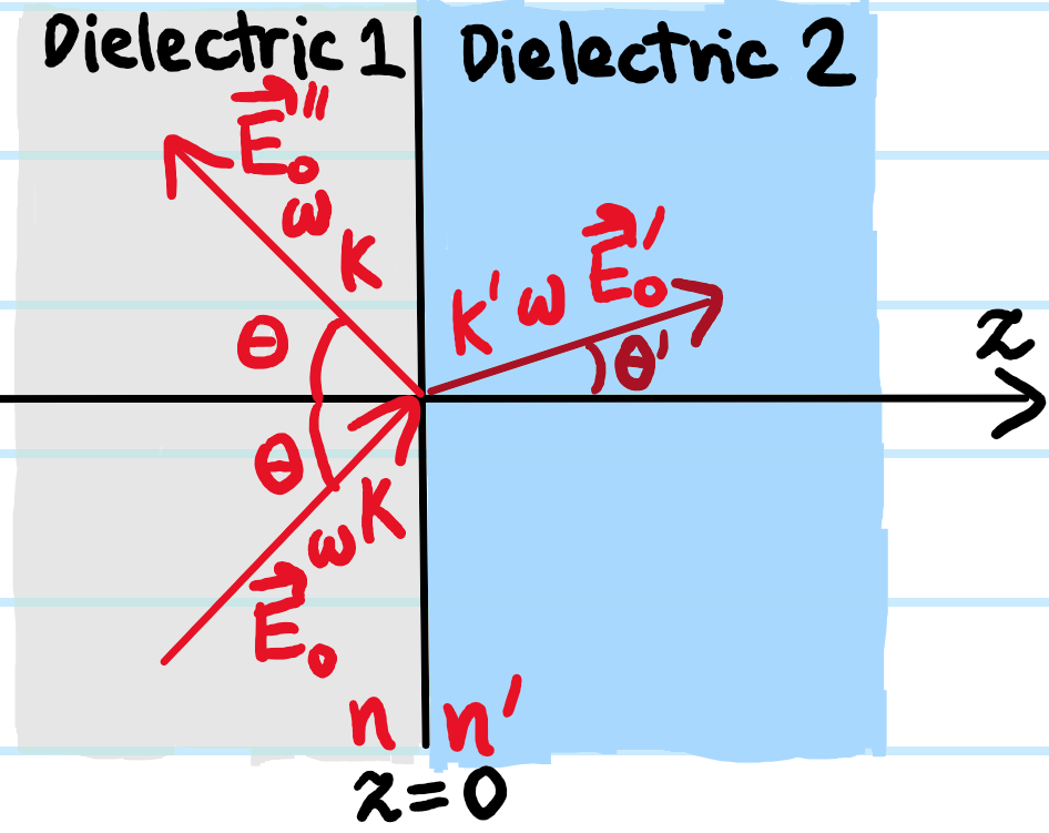
Solution #\(11\): The assumption of dielectrics is needed here in order to set \(\sigma_f=0\) and \(\textbf K_f=\textbf 0\) in the electromagnetic interface conditions (i.e. would not be true for conductors!). Note also that the amplitudes \(\textbf E_0,\textbf E’_0,\textbf E^{\prime\prime}_0\) are arbitrary, so capture all cases of linear, circular, or elliptical polarization.
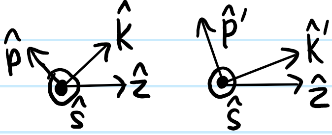
The incident wavevector is \(\textbf k=k\sin\theta\hat{\boldsymbol{\rho}}_{\phi}+k\cos\theta\hat{\textbf z}\) while the transmitted wavevector is \(\textbf k’=k’\sin\theta’\hat{\boldsymbol{\rho}}_{\phi}+k’\cos\theta’\hat{\textbf z}\); the incident electric field amplitude \(\textbf E_0\) lives in the orthogonal complement \(\text{span}^{\perp}(\textbf k)\) while \(\textbf E’_0\) lives in \(\text{span}^{\perp}(\textbf k’)\) (analogous remarks apply for the magnetic field amplitudes \(\textbf B_0,\textbf B’_0\) which are inseparably married to their respective electric fields but are not indicated on the diagram for simplicity). These two-dimensional subspaces admit convenient orthonormal bases given by the normal unit vector \(\hat{\textbf s}:=\hat{\textbf k}\times\hat{\textbf p}=\hat{\textbf k}’\times\hat{\textbf p}’\) and the parallel unit vectors \(\hat{\textbf p}:=\text{cot}\theta\hat{\textbf k}-\text{csc}\theta\hat{\textbf z}\) and likewise \(\hat{\textbf p}’:=\text{cot}\theta’\hat{\textbf k}’-\text{csc}\theta’\hat{\textbf z}\); here the words “normal” and “parallel” are with respect to the plane of incidence/transmission/reflection \(\text{span}(\textbf k,\hat{\textbf z})=\text{span}(\textbf k’,\hat{\textbf z})\).
By decomposing \(\textbf E_0=E_{0,s}\hat{\textbf s}+E_{0,p}\hat{\textbf p}\) where \(E_{0,s}=\textbf E_0\cdot\hat{\textbf s}\) and \(E_{0,p}=\textbf E_0\cdot\hat{\textbf p}\), and doing likewise for \(\textbf E’_0,\textbf E^{\prime\prime}_0,\textbf B_0,\textbf B’_0,\textbf B^{\prime\prime}_0\) and substituting all this into the \(4\) electromagnetic interface conditions with \(\hat{\textbf n}=\hat{\textbf z}\), one obtains the Fresnel equations:
\[t_s:=\frac{E’_{0,s}}{E_{0,s}}=\frac{2Y\cos\theta}{Y\cos\theta+Y’\cos\theta’}\]
\[r_s:=\frac{E^{\prime\prime}_{0,p}}{E_{0,p}}=\frac{Y\cos\theta-Y’\cos\theta’}{Y\cos\theta+Y’\cos\theta’}\]
\[t_p:=\frac{E’_{0,p}}{E_{0,p}}=\frac{2Y\cos\theta}{Y\cos\theta’+Y’\cos\theta}\]
\[r_p:=\frac{E^{\prime\prime}_{0,p}}{E_{0,p}}=\frac{Y\cos\theta’-Y’\cos\theta}{Y\cos\theta’+Y’\cos\theta}\]
where the admittances are \(Y:=Z^{-1}=\sqrt{\varepsilon/\mu}\) and likewise \(Y’:=Z’^{-1}=\sqrt{\varepsilon’/\mu’}\). Note here that all \(4\) coefficients \(t_s,r_s,t_p,r_p\) are defined here with respect to the electric field; one could have also defined them from the \(s\) and \(p\)-polarized components of the magnetic field, leading to almost the same Fresnel equations (differing by some subtle minus signs here and there).
Problem #\(12\): Sketch graphs of \(t_s,r_s,t_p,r_p\) as a function of the incident angle \(\theta\) in the two cases \(Y>Y’\) and \(Y<Y’\), and comment.
Solution #\(12\): From air to glass \(Y’/Y\approx 1.5\) (assuming both have \(\mu=\mu’=\mu_0\)):
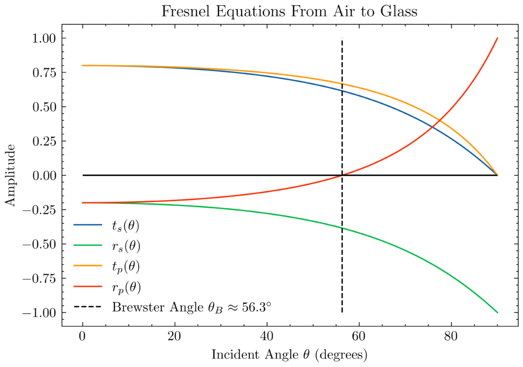
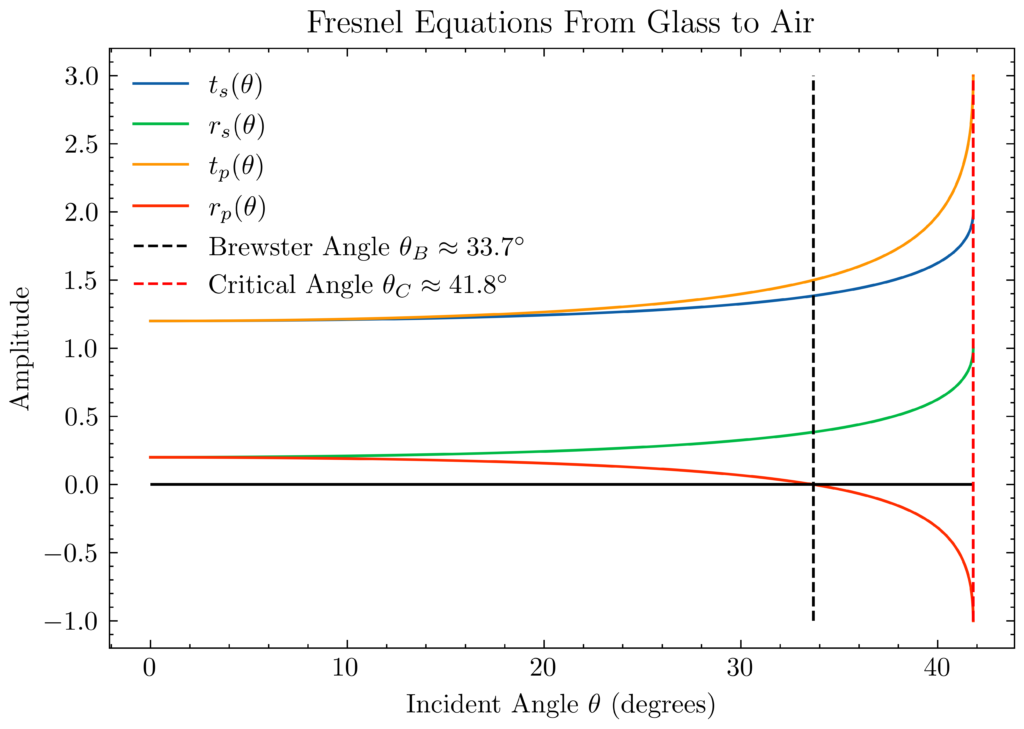
At normal incidence \(\theta=\theta’=0\), there is clearly no longer any distinction between \(s\) and \(p\)-polarization, reflecting the fact that (as is clear from the graph) \(t_s(\theta=0)=t_p(\theta=0)\) and \(r_s(\theta=0)=r_p(\theta=0)\) regardless of whether \(Y<Y’\) or \(Y>Y’\). In addition, again regardless of whether \(Y<Y’\) or \(Y>Y’\), there always exists a Brewster angle \(\tan\theta_B=\sqrt{\frac{1-(Y’/Y)^2}{(n/n’)^2-1}}\approx Y’/Y\) (approximation valid for non-magnetic dielectrics e.g. air, glass for which \(Y’/Y\approx n’/n\) and the reflected light \(\textbf k’\cdot\textbf k^{\prime\prime}=0\) is orthogonal to the refracted light \(\theta_B+\theta’_B\approx \pi/2\)) and is entirely linearly \(s\)-polarized since \(r_p(\theta=\theta_B)=0\). However, only in the case \(Y>Y’\) of going from an optically dense to less dense medium does there exist a critical angle \(\theta_C=\arcsin(Y’/Y)\) beyond which \(\theta>\theta_C\) only total internal reflection occurs together with transmission of an evanescent wave \(\textbf E'(\rho,\phi,z)=\textbf E’_0e^{-\sqrt{k^2\sin^2\theta-k’^2}z}e^{i(k\rho\cos(\phi-\phi_{\textbf k})\sin\theta-\omega t)}\).
Problem #\(13\): Building off of Problem #\(12\), calculate the transmitted powers \(T_s(\theta),T_p(\theta)\) along with the reflected powers \(R_s(\theta),R_p(\theta)\) as a function of incident angle \(\theta\) for both \(s\) and \(p\)-polarization. Verify that \(T_s(\theta)+R_s(\theta)=T_p(\theta)+R_p(\theta)=1\). Show that for air-to-glass at normal incidence (so that there is no distinction between \(s\) and \(p\)-polarization), \(R(\theta=0)\approx 4\%\).
Solution #\(13\): As long as one remembers the expression for the (period-averaged) Poynting vector \(\textbf S=\frac{1}{2}\textbf E\times\textbf H^*=\frac{Y|\textbf E_0|^2}{2}\hat{\textbf k}\), then the rest is easy (by definition the coefficients here are defined relative to the normal \(\hat{\textbf n}=\hat{\textbf z}\) of the interface though Poynting’s theorem with \(\textbf J_f=\textbf 0\) would hold in an arbitrary direction; there is also a nice way to see why this is using notions of “beam divergence”).
\[T_s(\theta)=\frac{\textbf S’_s\cdot\hat{\textbf z}}{\textbf S_s\cdot\hat{\textbf z}}=\frac{Y’\cos\theta’}{Y\cos\theta}|t_s(\theta)|^2\]
\[R_s(\theta)=\frac{\textbf S^{\prime\prime}_s\cdot\hat{\textbf z}}{\textbf S_s\cdot\hat{\textbf z}}=|r_s(\theta)|^2\]
\[T_p(\theta)=\frac{\textbf S’_p\cdot\hat{\textbf z}}{\textbf S_p\cdot\hat{\textbf z}}=\frac{Y’\cos\theta’}{Y\cos\theta}|t_p(\theta)|^2\]
\[R_p(\theta)=\frac{\textbf S^{\prime\prime}_p\cdot\hat{\textbf z}}{\textbf S_p\cdot\hat{\textbf z}}=|r_p(\theta)|^2\]
the rest is easy to check (aside: given the \(4\) electromagnetic boundary conditions earlier, can one write down some corresponding boundary conditions on \(\hat{\textbf n}\cdot\Delta\textbf S\) and \(\hat{\textbf n}\times\Delta\textbf S\) which capture energy conservation? Especially the first one seems to just coming from Poynting’s theorem).
Problem #\(14\): Using the Lorentz oscillator model of the electron \(e^-\), show how the atomic polarizability \(\alpha\), the electric susceptibility \(\chi_e\), the permittivity \(\varepsilon\), and the wavenumber \(k\) all become complex-valued functions of the frequency \(\omega\in\textbf R\) of the incident light.
Solution #\(14\): The equation of motion for the electron is taken to be of the usual form of a damped, driven harmonic oscillator:
\[\ddot{\textbf x}(t)+\Delta\omega\dot{\textbf x}(t)+\omega_0^2\textbf x(t)=\frac{q\textbf E_0}{m}e^{i(\textbf k_{\omega}\cdot\textbf x(t)-\omega t)}\]
where the damping coefficient \(\Delta\omega\) and the resonant frequency \(\omega_0\) are both phenomenological parameters of the Lorentz model (the former \(\Delta\omega\) is the quantum line width of the relevant optical transitions that have energy commensurate with \(\hbar\omega\), equivalently the spontaneous emission rate or reciprocal lifetime, while the latter \(\omega_0^2=q^2/4\pi\varepsilon_0ma^3\) has a classical form following Solution #\(1\)). Although of course the electric field \(\textbf E(\textbf x,t)=\textbf E_0e^{i(\textbf k_{\omega}\cdot\textbf x-\omega t)}\) of course has an accompanying magnetic field \(\textbf B(\textbf x,t)=\textbf B_0e^{i(\textbf k_{\omega}\cdot\textbf x-\omega t)}\), the magnetic force \(q\dot{\textbf x}\times\textbf B\) can be ignored in the non-relativistic limit \(|\dot{\textbf x}|\ll c\).
Making the further assumption that at the relevant frequency \(\omega\), \(\textbf k_{\omega}\cdot\textbf x(t)\ll 1\) at all times \(t\), then it really reduces to a linearly damped, driven harmonic oscillator, for which the steady state particular integral oscillation is:
\[\textbf x=\frac{q}{m}\frac{1}{\omega_0^2-\omega^2-i\omega\Delta\omega}\textbf E\]
Optionally multiplying this solution \(\textbf x\) by the electron charge \(q\), one can write the electric dipole moment of an atom as:
\[\textbf p=\frac{q^2}{m}\frac{1}{\omega_0^2-\omega^2-i\omega\Delta\omega}\textbf E\]
But from the definition \(\textbf p=\alpha\textbf E\), one immediately recognizes the atomic polarizability has become a \(\textbf C\)-valued function of \(\omega\in\textbf R\):
\[\alpha(\omega)=\frac{q^2}{m}\frac{1}{\omega_0^2-\omega^2-i\omega\Delta\omega}\]
From \(\textbf p\), one can get \(\textbf P\) through a factor of the number density \(n\) of electrons (equivalent to the number density of electric dipole moments):
\[\textbf P=n\textbf p=n\alpha\textbf E:=\varepsilon_0\chi_e\textbf E\]
So:
\[\chi_e(\omega)=\frac{\omega_p^2}{\omega_0^2-\omega^2-i\omega\Delta\omega}\]
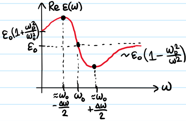
where the plasma frequency \(\omega_p^2=nq^2/m\varepsilon_0\) scales with the plasma density \(n\). The \(\textbf C\)-valued nature of the permittivity is then evident from \(\varepsilon(\omega)=\varepsilon_0(1+\chi_e(\omega))\) whose the real and imaginary parts are:
\[\Re\varepsilon(\omega)=\varepsilon_0\left(1-\frac{\omega_p^2(\omega^2-\omega_0^2)}{(\omega^2-\omega_0^2)^2+\omega^2\Delta\omega^2}\right)\]
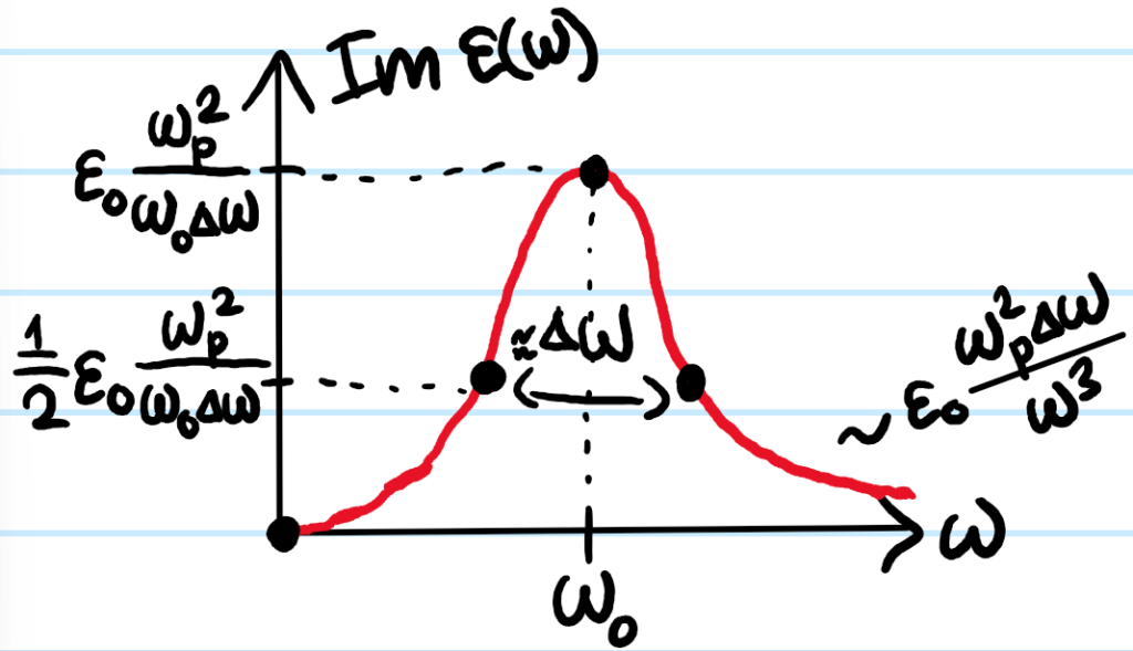
\[\Im\varepsilon(\omega)=\varepsilon_0\frac{\omega_p^2\omega\Delta\omega}{(\omega^2-\omega_0^2)^2+\omega^2\Delta\omega^2}\]
And the shape of both of their graphs is a good thing to get familiar with (note the roles played by the \(3\) distinct frequency scales in the function \(\omega_p,\omega_0,\Delta\omega\)):
As an aside, because the complexified \(\varepsilon(\omega)\) is complex analytic in the upper half-plane \(\Im\omega>0\) on causality grounds, its real and imaginary parts \(\Re\varepsilon(\omega),\Im\varepsilon(\omega)\) are related by Kramers-Kronig relations:
\[\Re\varepsilon(\omega)=\mathcal P\int_{-\infty}^{\infty}\frac{d\omega’}{\pi}\frac{\Im\varepsilon(\omega’)}{\omega’-\omega}\]
\[\Im\varepsilon(\omega)=\mathcal P\int_{-\infty}^{\infty}\frac{d\omega’}{\pi}\frac{\Re\varepsilon(\omega’)}{\omega-\omega’}\]
Problem #\(15\): Dispersion relations for waves are conventionally thought of as \(\omega=\omega_{\textbf k}\), but one can of course invert this to obtain \(\textbf k=\textbf k_{\omega}\) and view that as the dispersion relation. This view will be more useful here; think of the frequency \(\omega\in\textbf R\) as free real parameter one gets to select as the experimentalist.
For a linear dielectric in the absence of (free) charges or (free conduction) currents, what consequences does \(\varepsilon(\omega)\in\textbf C\) have for the propagation of light in such a medium?
Solution #\(15\): One always has the “naive linear” nondispersion:
\[|\textbf k_{\omega}|=\sqrt{\mu\varepsilon}\omega\]
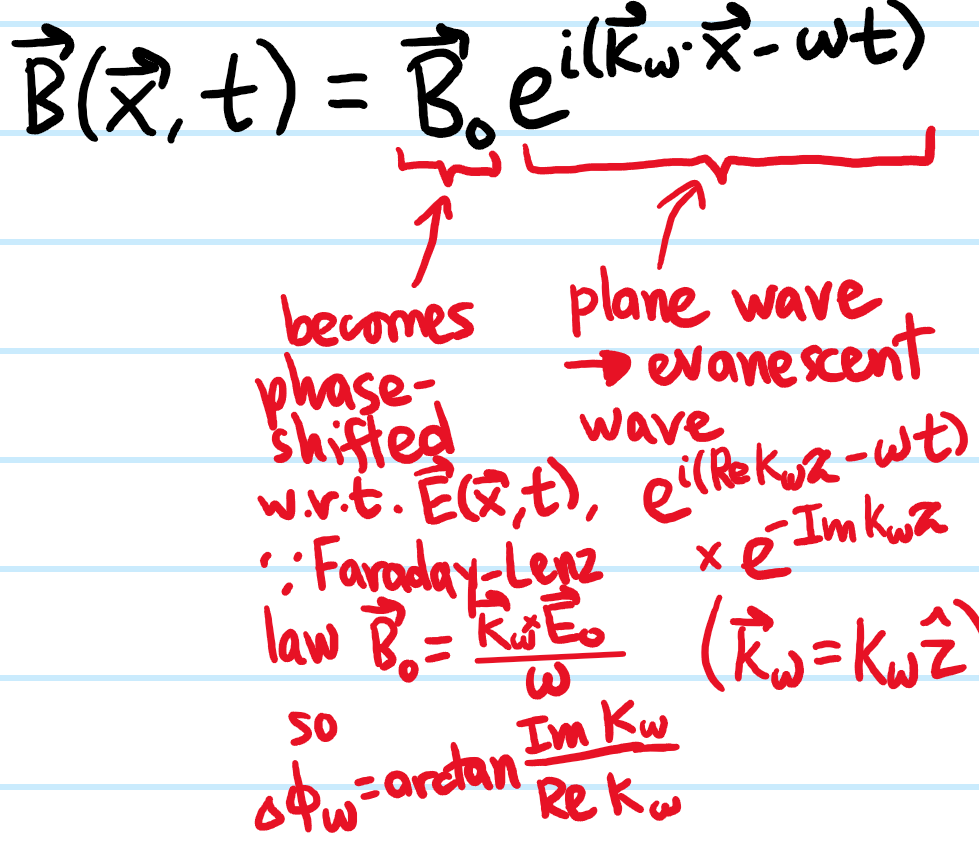
However, even though one typically assumes \(\mu\in\textbf R\) to be \(\omega\)-independent, the fact that \(\varepsilon=\varepsilon(\omega)\in\textbf C\) promotes the wavevector \(\textbf k_{\omega}\in\textbf C^3\) rather than the usual \(\textbf k_{\omega}\in\textbf R^3\). There are \(2\) important consequences of this, illustrated for instance using \(\textbf B(\textbf x,t)\):
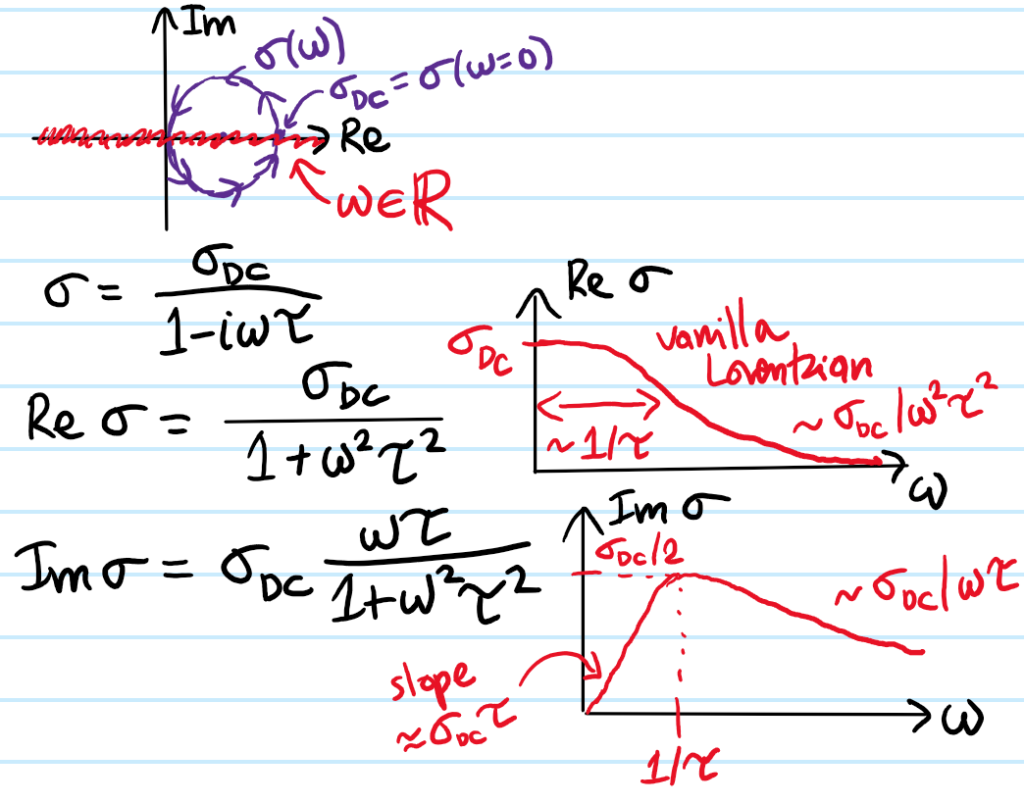
Problem #\(16\): Show using the Drude model that all of the discussion for dielectrics applies equally well to conductors provided the permittivity receives an additional \(\textbf C\)-contribution from conduction electrons of the form:
\[\varepsilon(\omega)\mapsto\varepsilon_{\text{eff}}(\omega):=\varepsilon(\omega)+\frac{i\sigma(\omega)}{\omega}\]
where the optical conductivity is given by the Mobius transformation:
\[\sigma(\omega)=\frac{\sigma_{\text{DC}}}{1-i\omega\tau}\]
where \(\sigma_{\text{DC}}=\sigma(\omega=0)=nq^2\tau/m=\varepsilon_0\tau\omega_p^2\) and \(\tau>0\) is the relaxation time between electron collisions.
Solution #\(16\): Now the equation of motion is basically the same as from the Lorentz oscillator model except there is no Hookean restoring force \(\omega_0=0\) and one renames \(\Delta\omega=1/\tau\). Notably, because the ODE is now merely \(1^{\text{st}}\)-order:
\[\dot{\textbf v}+\frac{1}{\tau}\textbf v=\frac{q\textbf E}{m}\]
The steady state particular integral velocity response \(\textbf v(t)=\textbf v_0e^{-i\omega t}\) to an AC electric field \(\textbf E=\textbf E_0e^{-i\omega t}\) is now a Mobius rather than a Lorentzian:
\[\textbf v=\frac{q\tau}{m}\frac{1}{1-i\omega\tau}\textbf E\]
In order to get optical conductivity \(\sigma(\omega)\), one just has to remember what its defining equation is in the first place, i.e. Ohm’s law \(\textbf J=\sigma\textbf E\). So computing \(\textbf J=\rho\textbf v=\frac{nq^2\tau}{m}\frac{1}{1-i\omega\tau}\textbf E\), the claim follows.
In Fourier space, applying Ohm’s law (valid for low mean free path of the electrons) and the continuity equation for local charge conservation, Maxwell’s equations in an ohmic conductor:
\[i\textbf k_{\omega}\cdot\varepsilon\textbf E_0=\frac{\textbf k_{\omega}\cdot\sigma\textbf E_0}{\omega}\]
\[i\textbf k_{\omega}\cdot\textbf B_0=0\]
\[i\textbf k_{\omega}\times\textbf E_0=-(-i\omega\textbf B_0)\]
\[i\textbf k_{\omega}\times\frac{\textbf B}{\mu}=\sigma\textbf E_0-i\omega\varepsilon\textbf E_0\]
And in particular, the last equation (Ampere-Maxwell) gives the desired \(\varepsilon_{\text{eff}}=\varepsilon+i\sigma/\omega\) (interestingly this same quantity is required to be non-vanishing \(\varepsilon_{\text{eff}}\neq 0\) so that Gauss’s law for the \(\textbf D\)-field yields transverse EM waves). Computing the usual \(\textbf k_{\omega}\times(\textbf k_{\omega}\times\textbf E_0)\) gives the dispersion relation:
\[k_{\omega}=\sqrt{\mu\varepsilon_{\text{eff}}}\omega\]
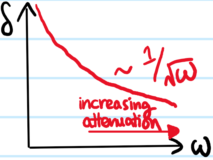
Problem #\(17\): How do waves behave in the low-\(\omega\) and high-\(\omega\) limits inside the conductor?
Solution #\(17\): For low-\(\omega\), the conductivity term dominates so the permittivity \(\varepsilon_{\text{eff}}\approx\varepsilon_0\frac{i\sigma}{\omega}\approx\varepsilon_0\frac{i\sigma_{\text{DC}}}{\omega}\) is purely imaginary. The dispersion relation then dictates:
\[k_{\omega}=\sqrt{\mu\varepsilon_{\text{eff}}}\omega=\sqrt{\frac{\mu\sigma_{\text{DC}}\omega}{2}}(1+i)\]
where the other option \(\sqrt{i}=-(1+i)/\sqrt{2}\) is rejected because one requires on physical grounds an evanescent wave so \(\Im k_{\omega}>0\). Moreover, because \(\Re k_{\omega}=\Im k_{\omega}\) in this case, the \(\textbf E\) (equivalently, roughly \(\textbf D\)) and \(\textbf B\) (equivalently \(\textbf H\)) fields are \(45^{\circ}\) out of phase in the conductor. All of the EM fields \(\textbf E,\textbf B,\textbf D,\textbf H\) are exponentially attenuated:
\[(\text{phasor})e^{i(\textbf k_{\omega}\cdot\textbf x-\omega t)}=(\text{phasor})e^{-z/\delta(\omega)}e^{i(z/\delta(\omega)-\omega t)}\]
where the skin depth \(\delta(\omega):=\sqrt{2/\mu\sigma_{\text{DC}}\omega}=\lambda/2\pi\) is on the order of a single wavelength \(\lambda\)!
For high-\(\omega\), \(\varepsilon\to\varepsilon_0(1-\omega_p^2/\omega^2)\) and \(\sigma\to i\sigma_{\text{DC}}/\omega\tau\) (just look at the graphs from earlier to see all of this!) so:
\[\varepsilon_{\text{eff}}\to\varepsilon_0\left(1-\frac{2\omega_p^2}{\omega_0^2}\right)\in\textbf R\]
The implication of this is that \(\omega_p\) (or more precisely \(\sqrt{2}\omega_p\)) provides a strict cut-off:
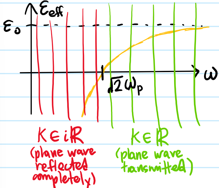
The atmosphere can be modelled as such a plasma and this underlies why FM radio waves with \(\omega>\sqrt{2}\omega_p\) transmit through the atmosphere whereas AM radio waves with \(\omega<\sqrt{2}\omega_p\) are reflected.