
The purpose of this post is to describe the Aharanov-Bohm phase and its relevance to Dirac’s classic \(1931\) argument for the quantization of magnetic charge (if magnetic monopoles were to exist) using the principles of quantum mechanics. Finally, a few more proofs of Dirac quantization will be given that were subsequently discovered.
Aharanov-Bohm Effect
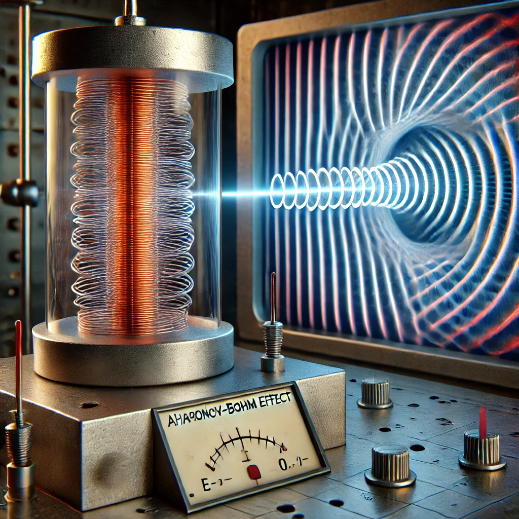
Here is ChatGPT’s depiction of the effect:
A simple idealized example that gets to the essence of the Aharanov-Bohm effect is as follows; consider a cylindrical magnetic flux tube \(\Phi_{\textbf B}\) (perhaps from some solenoid), and consider a charge \(q\) confined to move on a circle \(S^1_R\) of radius \(R\) outside the magnetic flux tube where \(\textbf B=\textbf 0\) (aside: from Maxwell’s equations \(\partial_{\textbf x}\cdot\textbf E=\partial_{\textbf x}\times\textbf E=\dot{\textbf E}=0\) outside the solenoid, so by the Helmholtz decomposition theorem I believe that \(\textbf E=\textbf 0\) outside the solenoid but I might be wrong about this). Despite this, the magnetic vector potential \(\textbf A\) cannot be zero due to Stokes’s theorem \(\Phi_{\textbf B}=\oint_{\textbf x\in S^1_R}\textbf A(\textbf x)\cdot d\textbf x\) which in a suitable gauge implies the azimuthally-circulating vector field \(\textbf A=\frac{\Phi_{\textbf B}}{2\pi R}\hat{\boldsymbol{\phi}}_{\phi}\). The Hamiltonian for this charge is (remember again it’s confined to the circle \(S^1_R\)):
\[H=\frac{(P_{\phi}-q\Phi_{\textbf B}/2\pi R)^2}{2m}\]
Since the particle is constrained to move on a circle, \(L_3=RP_{\phi}\), so:
\[H=\frac{(L_3-q\Phi_{\textbf B}/2\pi)^2}{2I}\]
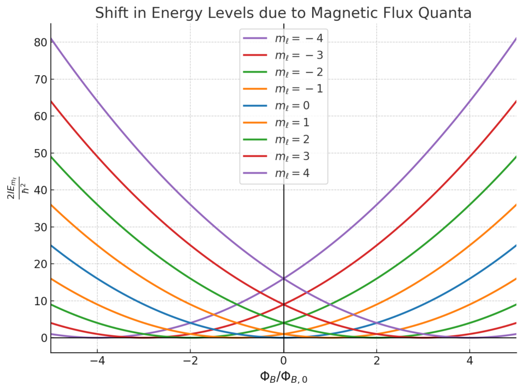
with \(I:=mR^2\) the moment of inertia. The energies are therefore quantized by \(m_{\ell}\in\textbf Z\):
\[E_{m_{\ell}}=\frac{\hbar^2}{2I}\left(m_{\ell}-\frac{\Phi_{\textbf B}}{\Phi_{\textbf B,0}}\right)^2\]
with the quantum of magnetic flux \(\Phi_{\textbf B,0}=h/e\). The corresponding usual \(L_3\)-eigenstate wavefunctions that we’ve known since we analyzed the “particle on a ring” back in the good ol’ days are all maximally delocalized and given by:
\[\langle\phi|E_{m_{\ell}}\rangle=\frac{1}{\sqrt{2\pi R}}e^{im_{\ell}\phi}\]
Anyways, focusing back on the energies \(E_{m_{\ell}}\), it is clear that the spectrum of the Hamiltonian \(H\) is indistinguishable within residue classes of the form \(\Phi_{\textbf B}\text{ mod }\Phi_{\textbf B,0}\) for any \(\Phi_{\textbf B}\in\textbf R\). Graphically, if one plots for various values of \(m_{\ell}\in\textbf Z\) the energy \(E_{m_{\ell}}\) as a function of \(\Phi_{\textbf B}/\Phi_{\textbf B,0}\), one obtains a sequence of parabolas (only \(-4\leq m_{\ell}\leq 4\) are shown but it’s important to realize that other parabola segments should be leaking into here too forming a lattice-like structure which would graphically explain the above observation about indistinguishability):
However, notice that the zero vector potential \(\textbf 0=\textbf A-\frac{\partial\Gamma}{\partial\textbf x}\) can (despite our earlier emphasis that \(\textbf A\neq\textbf 0\)!) be obtained from the earlier vector potential \(\textbf A(\rho,\phi)=\frac{\Phi_{\textbf B}}{2\pi \rho}\hat{\boldsymbol{\phi}}_{\phi}\) via the multivalued gauge transformation \(\Gamma(\phi)=\frac{\Phi_{\textbf B}\phi}{2\pi}\) (which means that \(\frac{\partial}{\partial\textbf x}\times\textbf A=\textbf 0\) is irrotational despite the fact that \(\textbf A\) appears azimuthally circulating) and therefore our earlier wavefunctions also transform accordingly into \(\frac{1}{\sqrt{2\pi R}}e^{im_{\ell}\phi}\mapsto \frac{1}{\sqrt{2\pi R}}e^{im_{\ell}\phi-iq\Gamma(\phi)/\hbar}\). Although it’s okay for the gauge \(\Gamma\) to be multivalued, it’s not okay on physical grounds for wavefunctions to be multivalued (i.e. they have to actually be functions!) and so the only way to ensure that the new wavefunctions are single-valued is iff \(\Phi_{\textbf B}/\Phi_{\textbf B,0}\in\textbf Z\). Thus, the gauge transformation is allowed iff the energy spectrum \(E_{m_{\ell}}\) is unaffected, meaning the quantum particle is completely oblivious to the magnetic flux tube’s existence. Thus, the restriction that the particle’s wavefunction \(\langle\phi|E_{m_{\ell}}\rangle\) has to wind \(\langle\phi+2\pi|E_{m_{\ell}}\rangle=\langle\phi|E_{m_{\ell}}\rangle\) around the flux tube \(\Phi_{\textbf B}\) is an example of how the topology of a space can have important quantum mechanical ramifications.
Double-Slit Experiment Using Classical Physics
Here we first recall how the far-field (also called the Fraunhofer) period-averaged interference pattern for the classic double-slit experiment is calculated classically using the usual wave theory of light. As usual, a monochromatic, coherent electromagnetic plane wave (polarized along the \(\hat{\textbf k}\) direction) with wavenumber \(k\) is incident normally on two infinitely thin slits separated by distance \(\Delta x\). From each slit emerges (via the magic wand of diffraction, or more precisely via the Huygens-Fresnel principle) monochromatic, coherent electromagnetic cylindrical waves of the same wavenumber \(k\) which interfere with each other everywhere in three-dimensional space \(\textbf R^3\). However, as is standard, we place a screen normally at a far distance \(\Delta y\gg k\Delta x^2\) away, thereby sampling a two-dimensional cross-section \(\cong\textbf R^2\subseteq\textbf R^3\) of the full three-dimensional space where all the interference is really happening (rant: in everyday usage the word interference generally brings with it a negative connotation, however we know that at various points \(\textbf x\in\textbf R^3\) in space waves can “interfere” not just in a destructive way befitting of the negative connotation but also in a constructive way which sort of lends itself to a cognitive dissonance. A more neutral synonym for interference would be superposition, and maybe a better name for interferometer would be superpositionometer but since it’s standard to speak about interference I’ll just stick to that annoying terminology).
To compute the time-averaged far-field interference pattern (here defined as the irradiance received by the screen) \(\bar I^{\infty}(x|k,\Delta x,\Delta y)\) at some position \(\textbf x=(x,\Delta y)\) on the screen \(y=\Delta y\), we first note that the two slits are located at \(\textbf x_{\pm}=(\pm\Delta x/2,0)\). If we arbitrarily focus for a moment on the far-field electric field \(\textbf E_+^{\infty}(\textbf x,t)\) associated with the cylindrical EM-wave emanating from just the slit at position \(\textbf x_+\), it is intuitively given by \(\textbf E_+^{\infty}(\textbf x,t)\sim E_0\cos k(|\textbf x-\textbf x_+|-ct)\hat{\textbf k}\). Because we’re dealing with cylindrical waves, the coefficient \(E_0\) is not actually a constant but rather exhibits the far-field decay \(E_0=E_0(|\textbf x-\textbf x_+|)\sim \frac{1}{\sqrt{|\textbf x-\textbf x_+|}}\) characteristic of Bessel function cylindrical waves. Nonetheless, we will ignore this amplitude attenuation in the electric field strength \(|\textbf E_+^{\infty}(\textbf x,t)|\) as it would distract from the important features (e.g. locations of bright and dark fringes) in the far-field interference pattern \(\bar I^{\infty}(x|k,\Delta x,\Delta y)\) itself which don’t depend on it.
Similarly, for the slit at \(\textbf x_-\), the far-field electric field “spilling out” of it is \(\textbf E_-^{\infty}(\textbf x,t)\sim E_0\cos k(|\textbf x-\textbf x_-|-ct)\hat{\textbf k}\) (importantly no phase shift term needs to be introduced in the argument of the \(\cos\) function because the plane wave was taken to be incident normally/simultaneously on both of the slits). The net far-field electric field therefore arises by interference \(\textbf E^{\infty}(\textbf x,t)=\textbf E_+^{\infty}(\textbf x,t)+\textbf E_-^{\infty}(\textbf x,t)\) and evaluating it at a point \(\textbf x=(x,\Delta y)\) on the screen yields (with the help of a trig identity):
\[\textbf E^{\infty}(\textbf x,t)=2E_0\cos \frac{k}{2}\left((|\textbf x-\textbf x_+|+|\textbf x-\textbf x_-|)-2ct\right)\cos\frac{k}{2}(|\textbf x-\textbf x_+|-|\textbf x-\textbf x_-|)\hat{\textbf k}\]
The far-field (but not yet period-averaged) irradiance \(I^{\infty}(\textbf x,t)\) received is given by the magnitude of the asymptotic Poynting field \(\textbf S^{\infty}\) (strictly projected onto the flat screen, though in the small-angle approximation we can assume this is roughly satisfied) \(I^{\infty}(\textbf x,t)\approx |\textbf S^{\infty}(\textbf x,t)|=\frac{|\textbf E^{\infty}(\textbf x,t)|^2}{\mu_0 c}=\frac{4E_0^2\cos^2\frac{k}{2}\left((|\textbf x-\textbf x_+|+|\textbf x-\textbf x_-|)-2ct\right)\cos^2\frac{k}{2}(|\textbf x-\textbf x_+|-|\textbf x-\textbf x_-|)}{\mu_0 c}\)
Now then, period-averaging \(\bar I^{\infty}(\textbf x)=\frac{ck}{2\pi}\int_0^{2\pi/ck} I^{\infty}(\textbf x,t)dt\) turns the time-dependent \(\cos^2\mapsto\frac{1}{2}\) so the final result is:
\[\bar I^{\infty}(\textbf x)=\frac{2E_0^2}{\mu_0 c}\cos^2\frac{k\Delta(\textbf x|\textbf x_+,\textbf x_-)}{2}\]
where the path-length difference is \(\Delta(\textbf x|\textbf x_+,\textbf x_-):=|\textbf x-\textbf x_+|-|\textbf x-\textbf x_-|\). The part where the far-field approximation is used has nothing to with the physics of interference or diffraction, and is just a matter of being able to simplify the path-length difference \(\Delta(\textbf x|\textbf x_+,\textbf x_-)\approx \Delta x\sin\theta\). This follows either from the standard geometric argument, or algebraically by approximating and binomial-expanding the metric \(|\textbf x-\textbf x_{\pm}|=\sqrt{|\textbf x|^2-2\textbf x\cdot\textbf x_{\pm}+|\textbf x_{\pm}|^2}\approx \sqrt{|\textbf x|^2-2\textbf x\cdot\textbf x_{\pm}}=\sqrt{|\textbf x|^2\pm|\textbf x|\Delta x\sin\theta}=|\textbf x|\sqrt{1\pm\frac{\Delta x\sin\theta}{|\textbf x|}}\approx |\textbf x|\pm\frac{\Delta x\sin\theta}{2}\).
Double Slit Experiment Using Quantum Mechanics
It may seem like the double-slit experiment falls within the realm of classical physics because, as we’ve just shown above, some simple-minded classical reasoning gives the correct answer for the asymptotic, period-averaged irradiance distribution \(\bar I^{\infty}(\textbf x)\) on the screen, in agreement with experiments. Yet in fact the double-slit experiment was really a smoking gun for quantum mechanics. Here we’ll redo the calculation, this time using quantum mechanics to see that it agrees with the classical answer (though it will be apparent that the two calculations are really isomorphic to each other!). Basically, the fundamental premise now is that instead of electric fields \(\textbf E_{\pm}(\textbf x,t)\) interfering as was the case classically, it is the position space wavefunctions \(\psi_{\pm}(\textbf x,t)\) (i.e. the probability amplitudes) that interfere (a common but false way of saying it is that the “photons are interfering with each other”; actually one can do the experiment sending in one photon at a time and over time the interference pattern builds up as a statistical distribution; this means that in a laser light for instance with trillions of photons, it is not the photons that are interfering with each other, but rather the wavefunction of each individual photon is in some sense interfering with itself). Mathematically, an incident plane wave \(\psi_{\text{incident}}(x)=e^{ikx}\) diffracts into two cylindrical wavefunctions which interfere to produce the total scattered wavefunction \(\psi_{\text{scattered}}(x)=\psi_+(x)+\psi_-(x)=e^{ik|\textbf x-\textbf x_+|}+e^{ik|\textbf x-\textbf x_-|}\) (notice that all along we have simply ignored the time dependence as is customary for stationary states!). The probability density is therefore \(|\psi_{\text{scattered}}(x)|^2=|\psi_+(x)|^2+|\psi_-(x)|^2+2\Re(\psi_+(x)\psi_-^*(x))=2(1+\Re e^{ik\Delta(\textbf x|\textbf x_+,\textbf x_-)})=2(1+\cos k\Delta(\textbf x|\textbf x_+,\textbf x_-))\). The form of this result clearly agrees with the classical result, where the key was the interference term \(\Re(\psi_+(x)\psi_-^*(x))\) which wouldn’t be present if one were to just throw classical particles at the double slits.
There is also another nice way to think about it using Heisenberg’s uncertainty principle. We can imagine that at the moment when the photon is passing through one of the slits, it has an equal probability to pass through either of the slits and so is initially prepared in the symmetric “Schrodinger’s cat state” \(|\psi\rangle=\frac{|\textbf x_+\rangle+|\textbf x_-\rangle}{\sqrt 2}\). The fact that we initially know the particle’s position pretty well along the \(x\)-axis means by Heisenberg’s uncertainty principle that there would be a large uncertainty in its momentum \(P_1\) along the \(x\)-direction as it exits the slit; this wide distribution of possible momenta, together with the interference, can be seen to heuristically rationalize why an interference pattern so spread out is observed! More precisely, the wavefunction in momentum space is \(\langle\textbf p|\psi\rangle=\frac{\langle \textbf p|\textbf x_+\rangle+\langle \textbf p|\textbf x_-\rangle}{\sqrt 2}=\frac{e^{-i\textbf p\cdot\textbf x_+/\hbar}+e^{-i\textbf p\cdot\textbf x_-/\hbar}}{\sqrt{2h^3}}\) from which it is clear that computing the probability distribution \(|\langle\textbf p|\psi\rangle|^2\) will produce the same shape of the interference pattern (since \(\textbf x_{\pm}\) are both “along the \(x\)-axis”, it makes sense to also only consider momenta \(\textbf p\) lying along the \(x\)-axis too). Note in particular that any kind of detector which could tell you whether the photon passed through a given slit will also disturb the interference pattern by virtue of collapsing the wavefunction (note the screen can, in quantum mechanical terms, be thought of as a measuring device for the position observable \(X\)).
Examples: The above calculation therefore highlights how to solve for the far-field interference pattern on a flat screen in a diffraction setup from a general grating geometry; classically one computes the Fourier transform of the transparency \(T(\textbf x)\) of the grating whereas quantum mechanically one computes the momentum space wavefunction in the \(x\)-direction \(\psi(\textbf p_1)\) at the grating (which itself is the Fourier transform of the position space wavefunction \(\psi(\textbf x)\) at the grating). For instance, for a single slit of finite width \(\Delta x>0\) (note that we previously assumed the double slits were infinitely thin, here if we did the same then we wouldn’t get an interference pattern), if the photon is equally likely to pass anywhere within the slit region then \(\psi(x)=\frac{1}{\sqrt{\Delta x}}\) for \(x\in[-\Delta x/2,\Delta x/2]\) and vanishes in the \(V=\infty\) potential region (this is called a box or top-hat filter). The momentum space wavefunction is therefore \(\psi(p_1)\propto \int_{-\Delta x/2}^{\Delta x/2}e^{-ixp_1/\hbar}dx\propto\text{sinc}\frac{\Delta xp_1}{2\hbar}=\text{sinc}\frac{k_1\Delta x}{2}\). Thus, because \(k_1=k\sin\theta\), the irradiance distribution (which we see is really a statistical distribution of photon position \(X\)) is \(I^{\infty}(\theta|k,\Delta x)\propto |\psi(p_1=\hbar k_1)|^2\propto \text{sinc}^2\left(\frac{k\Delta x}{2}\sin\theta\right)\). If on the other hand one has a double slit where the centers of each slit are separated by \(\Delta x\) but the slits themselves are also not infinitely thin but rather have some width \(a\), then such a slit is simply the spatial convolution of the single slit of width \(a\) with the infinitely thin double slits separated by \(\Delta x\), so by the convolution theorem the far-field interference pattern of such a grating is the product of their individual far-field interference patterns \(\bar I^{\infty}(\theta)\propto\cos^2\left(\frac{k\Delta x}{2}\sin\theta\right)\text{sinc}^2\left(\frac{ka}{2}\sin\theta\right)\). As a corollary, if \(\Delta x=a\) then \(\bar I^{\infty}(\theta)\propto\cos^2\left(\frac{k\Delta x}{2}\sin\theta\right)\text{sinc}^2\left(\frac{ka}{2}\sin\theta\right)\propto\text{sinc}^2(ka\sin\theta)\) becomes a single slit of width \(2a\).
Double Slit Experiment with a Twist
Now consider placing a flux tube \(\Phi_{\textbf B}\) behind the double slits; how does this affect the far-field interference pattern? Well, since it’s just another flux tube, we already saw that the associated magnetic vector potential \(\textbf A\) circulates around it, yet remains irrotational and thus conservative with gauge \(\frac{\partial}{\partial\textbf x}\int_{\textbf x_0}^{\textbf x}\textbf A(\textbf x’)\cdot d\textbf x’=\textbf A(\textbf x)\) where \(\textbf x_0\in\textbf R^3\) is an arbitrary reference point for the line integral. Now then, the story starts the same, sending in an incident plane wave \(\psi_{\text{incident}}(x)=e^{ikx}\) which diffracts through the slits into scattered cylindrical waves that interfere \(\psi_{\text{scattered}}(x)=\psi_+(x)+\psi_-(x)=e^{ik|\textbf x-\textbf x_+|}+e^{ik|\textbf x-\textbf x_-|}\). But now, because we’re doing a gauge transformation \(\textbf A\mapsto\textbf 0\) via the gauge \(\int_{\textbf x_0}^{\textbf x}\textbf A(\textbf x’)\cdot d\textbf x’\) above, each wavefunction must transform by respective \(U(1)\) phases \(\psi_{\pm}(x)\mapsto e^{-iq\int_{\textbf x_{\pm}}^{\textbf x}\textbf A(\textbf x’)\cdot d\textbf x’/\hbar}\psi_{\pm}(x)\). Although the phases acquired by each wavefunction depends on what \(\textbf A\) is, and so isn’t gauge-invariant, the phase difference \(\frac{q}{\hbar}\oint_{\textbf x}\textbf A(\textbf x)\cdot d\textbf x=\frac{q\Phi_{\textbf B}}{\hbar}\) (which is what counts in the interference term \(\Re(\psi_+\psi_-^*)\)) is gauge invariant, and notably has the effect of translating the entire interference pattern either “left” or “right” proportional to the amount of magnetic flux \(\Phi_{\textbf B}\) applied in the flux tube (this is experimentally verified!). Thus, the Aharanov-Bohm phase associated to any magnetic flux \(\Phi_{\textbf B}\) is \(e^{2\pi i\Phi_{\textbf B}/\Phi_{\textbf B,0}}\in U(1)\). Clearly, it’s \(1\) if and only if \(\Phi_{\textbf B}/\Phi_{\textbf B,0}\in\textbf Z\), which again means that only when the magnetic flux is divisible into an integer number of quanta does the interference pattern look like the usual untranslated double-slit interference pattern.
Magnetic Monopoles
Recall that “electric monopoles” exist; they are basically point charges with electric charge \(q\in\textbf R\), or more precisely \(q\in e\textbf Z\) with \(e\approx 1.602\times 10^{-19}\text{ C}\) the elementary quantum of charge (ignoring quarks, etc.). The electrostatic field of such an electric monopole is the usual Coulomb field:
\[\textbf E=\frac{q}{4\pi\varepsilon_0r^2}\hat{\textbf r}\]
This result follows from the integral form of Gauss’s law for \(\textbf E\)-fields \(\Phi_{\textbf E,\partial V}=\frac{Q_V}{\varepsilon_0}\) with the suitable Gaussian surface \(S^2_r\). Meanwhile, we know that normally Gauss’s law for \(\textbf B\)-field simply says \(\Phi_{\textbf B,\partial V}=0\) for any volume \(V\). But if magnetic monopoles were to exist, this law would be (I don’t know how to rigorously justify this but it seems intuitively reasonable) \(\Phi_{\textbf B,\partial V}=G_V\) where \(G_V\) is now the magnetic charge enclosed in \(V\) (and has the same units as the magnetic flux, e.g. webers \(\text{Wb}\)). In particular, for a magnetic monopole of magnetic charge \(g\) (perhaps this symbol is chosen because it kind of looks dual to the usual symbol \(q\) for electric charge), it follows that the magnetic field is also Coulombic and given by:
\[\textbf B=\frac{g}{4\pi r^2}\hat{\textbf r}\]
However, it turns out that not just any magnetic monopole charge \(g\) is allowed by quantum mechanics. Dirac’s original argument was to consider an electric charge \(q\) that completes say a “counter-clockwise” circular loop \(S^1\) around a magnetic monopole \(g\) with the radial magnetic field \(\textbf B\) above. This causes the wavefunction (this is where the quantum mechanics comes in!) of \(q\) to acquire an Aharanov-Bohm phase \(e^{-iq\oint_{\textbf x\in S^1}\textbf A(\textbf x)\cdot d\textbf x/\hbar}\) where \(\textbf A\) is some we-don’t-know-if-it-even-exists vector potential for the radial magnetic field \(\textbf B\) of the monopole. By Stokes’ theorem, we have:
\[\oint_{\textbf x\in S^1}\textbf A(\textbf x)\cdot d\textbf x=\Phi_{\textbf B,S^2_N/2}=g/2\]
where \(S^2_N/2\) is the “northern” hemisphere oriented with outward normal. On the other hand, it is also \(-\Phi_{\textbf B,S^2_S/2}=-g/2\) by taking the southern hemisphere (although these two separate line integral computations should not be treated transitively because only the Aharanov-Bohm phase is observable/meaningful). This means:
\[e^{-iqg/2\hbar}=e^{iqg/2\hbar}\]
This forces the product of their respective charges \(qg\) must be a multiple of Planck’s constant \(qg\in h\textbf Z\), or equivalently \(g\in\Phi_{\textbf B,0}\textbf Z\) comes in multiples of the quantum flux. This is the Dirac quantization condition. For a pair of dyons \((q_1,g_1),(q_2,g_2)\) (thought of as “electromagnetic charges”), the Dirac-Zwanziger quantization condition is:
\[\det\begin{pmatrix}q_1 & g_1 \\ q_2 & g_2 \end{pmatrix}\in h\textbf Z\]
obtained by orbiting each dyon in the background of the other dyon. Above, the explicit construction of a magnetic vector potential \(\textbf A\) for the monopole magnetic field \(\textbf B\) was avoided. Can it even be done? The answer is yes, thanks to the fact that \(\textbf R^3-\{\textbf 0\}\) admits a topologically non-trivial \(U(1)\) bundle over \(S^2\) unlike \(\textbf R^3\). For instance, the following Dirac strings will do the trick:
\[\textbf A_{\text{Dirac string}}^{\pm}(r,\theta,\phi)=\pm\frac{g}{4\pi r}\frac{1\mp\cos\theta}{\sin\theta}\hat{\boldsymbol{\phi}}_{\phi}\]
they are singular gauge connections on the half-lines \(\theta=0,\pi\) respectively.
Angular Momentum Quantization Implies Dirac Quantization
If the above argument for the Dirac quantization condition was not sufficiently convincing, here is a better argument in my opinion. Consider fixing the magnetic monopole \(g\) at the origin, and asking about the classical dynamics of a charge \(q\) experiencing the Lorentz force \(\dot{\textbf{p}}=q\dot{\textbf x}\times\textbf B(\textbf x)\) of the monopole’s magnetic field \(\textbf B\). Since \(\textbf B\) is central, one might think that, similar to the situation for a central force, maybe angular momentum \(\textbf L=\textbf x\times\textbf p\) would be an interesting quantity to look at (though here it’s clearly not a central force!). Specifically, its time derivative can be computed as:
\[\dot{\textbf L}=\frac{d}{dt}\left(\frac{qg}{4\pi}\hat{\textbf r}\right)\]
So indeed \(\textbf L\) is not conserved, but the modified angular momentum \(\textbf L’:=\textbf L-\frac{qg}{4\pi}\hat{\textbf r}\) is thus conserved (think of the contribution term as the angular momentum in the electromagnetic field itself). The component of this modified angular momentum along the particle’s position vector is also conserved \(\textbf L’\cdot\hat{\textbf r}=-qg/4\pi\), suggesting motion constrained to a cone. But the angular momentum along any direction must be quantized (this is where the quantum mechanics sneaks in) as \(m\hbar\). The slight catch here is that \(m\) is not just restricted to integers (which is normally the case for orbital angular momentum), but can also be half-integers. Equating \(qg/4\pi\in\frac{\hbar}{2}\textbf Z\) reproduces the Dirac quantization condition.