
Problem: Define the \(2\) words in the phrase “ideal paramagnet“. Show that a classical ideal paramagnet of \(N\) spins each with the same fixed magnetic dipole moment \(\mu:=|\boldsymbol{\mu}|\) placed in a uniform external magnetic field \(B:=|\mathbf B|\) will develop a uniform non-zero induced average magnetization \(\langle M(B)\rangle=n\mu L(\beta\mu B)\) along the direction of \(\mathbf B\) where the Langevin function \(L(x):=\coth(x)-1/x\).
Solution: Ideal means the \(N\) spins are non-interacting with respect to each other (hence there’s no need to specify the precise geometric configuration of the \(N\) spins such as whether they’re on a lattice \(\Lambda\), etc.). Paramagnet imposes conditions on the first \(2\) Taylor expansion coefficients of \(\langle M(B)\rangle\) about \(B=0\):
- Non-magnetic/absence of spontaneous magnetization \(\langle M(B=0)\rangle=0\).
- Positive-definite zero-field magnetic susceptibility \(\chi_{\mu}/\mu_0:=\partial \langle M\rangle/\partial (B=0)>0\).
Classically, for a single classical spin, the state space is \((\theta,\phi)\in S^2\) and the \(\phi\)-independent Hamiltonian is \(H(\theta)=-\boldsymbol{\mu}\cdot\mathbf B=-\mu B\cos\theta\), so the single-spin partition function is:
\[Z_1=\int_{-1}^1d\cos\theta\int_0^{2\pi}d\phi e^{-\beta H(\theta)}=4\pi\text{sinhc}\beta\mu B\]
Thus, \(F_1=-k_BT\ln Z_1\) and \(\langle\mu_x\rangle=\langle\mu_y\rangle=0\) whereas:
\[\langle\mu_z\rangle=\int_{-1}^1d\cos\theta\int_0^{2\pi}d\phi\frac{e^{\beta\mu B\cos\theta}}{Z_1}\mu\cos\theta=\frac{\partial \ln Z_1}{\partial\beta B}=-\frac{\partial F}{\partial B}=\mu L(\beta\mu B)\]
and hence the result follows from \(\langle M(B)\rangle=n\langle\mu_z\rangle\) where \(n:=N/V\).
Problem: Show that in the high-temperature limit where \(x:=\beta\mu B\ll 1\), the Taylor expansion of the Langevin function about \(x=0\) is \(L(x)=x/3+O_{x\to 0}(x^3)\). Hence, derive Curie’s high-temperature ideal paramagnet law \(\chi_{\mu}=C/T\) for the zero-field magnetic susceptibility and state the value of the Curie constant \(C>0\).
Solution: One has:
\[L(x)=\coth x-\frac{1}{x}=\frac{\cosh x}{\sinh x}-\frac{1}{x}\approx\frac{1+x^2/2+…}{x+x^3/6}-\frac{1}{x}\]
\[=\frac{1}{x}\left(\frac{1+x^2/2}{1+x^2/6}-1\right)\approx\frac{1}{x}\left((1+x^2/2)(1-x^2/6)-1\right)=x/3+O_{x\to 0}(x^3)\]
Thus, it is straightforward to compute the Curie constant \(C=\mu_0 n\mu^2/3k_B\) for a classical ideal paramagnet.
Problem: Repeat the above analysis but for a quantum ideal paramagnet in which all \(N\) spins have the same fixed total angular momentum quantum number \(j\in\{0,1/2,1,…\}\).
Solution: Now, for a single quantum spin with state vector in the manifold \(\mathbf C^{2j+1}\), the spectrum of its Hamiltonian is given by the weak-field Zeeman splitting \(E_{|j,m_j\rangle}=g_jm_j\mu_BB\) for Landé \(g\)-factor \(g_j=1+\frac{j(j+1)+s(s+1)-\ell(\ell+1)}{2j(j+1)}\) and the canonical partition function is a Dirichlet kernel:
\[Z_1=\sum_{m_j=-j}^je^{-\beta E_{|j,m_j\rangle}}=\frac{\sinh(j+1/2)g_j\beta\mu_BB}{\sinh(g_j\beta\mu_BB/2)}\]
Repeating the same steps as above, this time one finds:
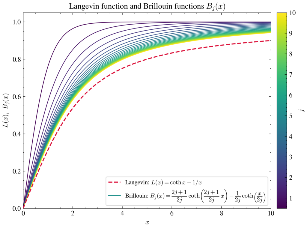
\[\langle M(B)\rangle=ng_jj\mu_B B_j(\beta g_jj\mu_BB)\]
where the Brillouin function is defined by:
\[B_j(x):=\left(1+\frac{1}{2j}\right)\coth\left(1+\frac{1}{2j}\right)x-\frac{1}{2j}\coth\frac{x}{2j}\]
In particular, as \(j\to\infty\), \(2j+1\to\infty\) and one recovers the classical continuous angle \(\theta\in [0,\pi]\) and \(\lim_{j\to\infty}B_j(x)=L(x)\).
This is consistent with the Taylor expansion \(B_j(x)=\frac{j+1}{3j}x+O_{x\to 0}(x^3)\) which leads to the quantum Curie constant \(C=\mu_0ng_j^2j(j+1)\mu_B^2/3k_B\). Instead of looking at \(j\to\infty\), one can also take the quantum limit \(j=s=1/2\) and \(\ell=0\), in which case \(g_j=2\) and:
\[B_{1/2}(x)=2\coth 2x-\coth x=\tanh x\]
so one recovers the familiar \(2\)-level system average magnetization \(\langle M\rangle=n\mu_B\tanh\beta\mu_BB\) with Curie constant \(C=\mu_0n\mu_B^2/k_B\).
Problem: Explain why classical statistical mechanics (when applied consistently!) predicts \(\langle\mathbf M(\mathbf B)\rangle=\mathbf 0\) for all \(\mathbf B\) (this is called the Bohr-van Leeuwen theorem). Since the Langevin derivation used a classical stat mech approach yet was able to predict a nontrivial \(\mathbf M(\mathbf B)\), explain why it doesn’t violate the BvL theorem.
Solution: The BvL theorem follows mathematically from the fact that the canonical \(N\)-particle partition function:
\[Z(\beta,\mathbf B)=\frac{1}{h^{3N}N!}\int d^3\mathbf x_1…d^3\mathbf x_Nd^3\mathbf p_1…d^3\mathbf p_Ne^{-\beta H}\]
with \(H=\sum_{i=1}^N\frac{|\mathbf p_i-q_i\mathbf A(\mathbf x_i)|^2}{2m_i}+V(\mathbf x_1,…,\mathbf x_N)\) can instead (via change of variables) be integrated over the kinetic momenta \(m_i\mathbf v_i:=\mathbf p_i-q_i\mathbf A(\mathbf x_i)\) rather than the canonical momenta \(\mathbf p_i\) without incurring a Jacobian penalty \(\partial (m_1\mathbf v_1,…,m_N\mathbf v_N)/\partial(\mathbf p_1,…,\mathbf p_N)=1\), so \(Z(\beta,\mathbf B)=Z(\beta,\mathbf B=\mathbf 0)\) is \(\mathbf B\)-independent and hence \(F=-k_BT\ln Z\) is also \(\mathbf B\)-independent, leading to the BvL theorem \(\langle\mathbf M\rangle=-V^{-1}\partial F/\partial\mathbf B=\mathbf 0\).
By assuming that one could speak of a “fixed magnetic dipole moment \(\mu\)” for all the atoms, Langevin was implicitly quantizing the system since in hindsight \(\mu=g_jj\mu_B\) and \(j\) is quantized and fixed (indeed, making the replacement \(\mu\mapsto g_jj\mu_B\) in the Langevin magnetization maps in the \(j\to\infty\) limit directly onto the Brillouin magnetization). As a result, it is better to regard the Langevin result for \(\langle M(B)\rangle\) as a semi-classical formula rather than strictly belonging to classical physics (otherwise it would violate the BvL theorem!).
Problem: State and prove the Stoner criterion \(\frac{g_V(E_F)}{2}g>1\) for itinerant ferromagnetism.
Solution: The Stoner criterion is derived within a toy model of itinerant ferromagnetism known fittingly as the Stoner model (a mean-field version of the Fermi-Hubbard model). That is, given a fixed number density \(n=n_{\uparrow}+n_{\downarrow}\) of spin-\(1/2\) fermions, each of these can be considered to form their own Fermi sea with \(E_{F,\uparrow}=\hbar^2(3\pi^2n_{\uparrow})^{2/3}/2m\) and similarly for \(E_{F,\downarrow}\). The total energy density \(\mathcal E\) of the system is then:
\[\mathcal E(n_{\uparrow},n_{\downarrow})=\frac{3}{5}n_{\uparrow}E_{F,\uparrow}+\frac{3}{5}n_{\downarrow}E_{F,\downarrow}+gn_{\uparrow}n_{\downarrow}-\mu(n_{\uparrow}+n_{\downarrow}-n)\]
Setting \(\partial\mathcal E/\partial n_{\uparrow}=\partial\mathcal E/\partial n_{\downarrow}=\partial\mathcal E/\partial\mu=0\) using the fact that \(nE_F\propto n^{5/3}\Rightarrow\partial (nE_F)/\partial n=5E_F/3\) leads to the system of equations:
\[E_{F,\uparrow}+gn_{\downarrow}=E_{F,\downarrow}+gn_{\uparrow}\]
\[n_{\uparrow}+n_{\downarrow}=n\]
The simplest (and in most circumstances, the unique) solution to these equations is the unpolarized paramagnetic occupation numbers \(n_{\uparrow}=n_{\downarrow}=n/2\) (and thus \(E_{F,\uparrow}=E_{F,\downarrow}:=E_F\)) as if the Stoner interaction \(g=0\) didn’t exist. So \((n_{\uparrow},n_{\downarrow})=(n/2,n/2)\) is always a stationary point of the function \(\mathcal E(n_{\uparrow},n_{\downarrow})\), but what about its stability? One can compute the Hessian matrix:
\[\begin{pmatrix}\partial^2\mathcal E/\partial n_{\uparrow}^2&\partial^2\mathcal E/\partial n_{\uparrow}\partial n_{\downarrow} \\ \partial^2\mathcal E/\partial n_{\uparrow}\partial n_{\downarrow} & \partial^2\mathcal E/\partial n_{\downarrow}^2\end{pmatrix}=\begin{pmatrix}\partial E_{F,\uparrow}/\partial n_{\uparrow} & g \\ g & \partial E_{F,\downarrow}/\partial n_{\downarrow}\end{pmatrix}=\begin{pmatrix} 2/g_V(E_F) & g \\ g & 2/g_V(E_F) \end{pmatrix}\]
using the fact that the total density of states per unit volume per spin \(g_{V,\uparrow}(E)=g_{V,\downarrow}(E)=g_V(E)/2\) are equal and sum to the total density of states per unit volume and moreover \(g_V(E_F)=\partial n/\partial E_F\). The eigenvectors of the Hessian are clearly \((1,1)\) and \((1,-1)\) from which one deduces the eigenvalues \(\frac{2}{g_V(E_F)}+g\) and \(\frac{2}{g_V(E_F)}-g\). Since both \(g_V(E_F),g>0\), the stationary point \((n_{\uparrow},n_{\downarrow})=(n/2,n/2)\) is thus an unstable saddle point iff the eigenvalue \(\frac{2}{g_V(E_F)}-g<0\) which rearranges to the standard form of the Stoner criterion \(\frac{g_V(E_F)}{2}g>1\).
Because \(\mathcal E(n_{\uparrow},n_{\downarrow})\) is a function of only \(2\) variables, the second partial derivative test asserts that this