
Problem: Let \(\boldsymbol{\Theta}\) be a smooth statistical manifold, and let \(D:\boldsymbol{\Theta}^2\to [0,\infty)\) be a smooth function. What does it mean for \((\boldsymbol{\Theta},D)\) to be a “divergence manifold“?
Solution: The notion of a divergence manifold relaxes the axioms of a metric space, specifically still demanding \(D(\boldsymbol{\theta} || \boldsymbol{\theta}’)\geq 0\) and \(D(\boldsymbol{\theta} || \boldsymbol{\theta}’)=0\Leftrightarrow\boldsymbol{\theta}’=\boldsymbol{\theta}\) for all \(\boldsymbol{\theta},\boldsymbol{\theta}’\in\boldsymbol{\Theta}\) but no longer enforcing symmetry \(D(\boldsymbol{\theta} || \boldsymbol{\theta}’)=D(\boldsymbol{\theta}’ || \boldsymbol{\theta})\) or the triangle inequality \(D(\boldsymbol{\theta} || \boldsymbol{\theta}^{\prime\prime})\leq D(\boldsymbol{\theta} || \boldsymbol{\theta}’) + D(\boldsymbol{\theta}’ || \boldsymbol{\theta}^{\prime\prime})\).
Problem: Explain how any divergence manifold \((\boldsymbol{\Theta},D)\) enjoys the free gift of being automatically equipped with a canonical Riemannian metric tensor field \(g_D(\boldsymbol{\theta}):T_{\boldsymbol{\theta}}(\boldsymbol{\Theta})^2\to\mathbf R\) induced by the divergence function \(D\).
Solution: The so-called Fisher information metric \(g_D(\boldsymbol{\theta})=(g_D)_{ij}(\boldsymbol{\theta})d\theta_i\otimes d\theta_j\) on the statistical manifold \(\boldsymbol{\Theta}\) induced by the divergence \(D\) is basically just its Hessian:
\[(g_D)_{ij}(\boldsymbol{\theta}):=\left(\frac{\partial^2 D(\boldsymbol{\theta}||\boldsymbol{\theta}’)}{\partial\theta’_i\partial\theta’_j}\right)_{\boldsymbol{\theta}’=\boldsymbol{\theta}}\]
Intuitively, one can think of the divergence \(D(\boldsymbol{\theta}||\boldsymbol{\theta}’)\) of \(\boldsymbol{\theta}’\in\boldsymbol{\Theta}\) from \(\boldsymbol{\theta}\in\boldsymbol{\Theta}\) as holding the “ground truth” distribution \(\boldsymbol{\theta}\) fixed while sniffing around for a proxy distribution \(\boldsymbol{\theta}’\) to approximate \(\boldsymbol{\theta}\). By the axioms of a divergence manifold, the global minimum value \(D(\boldsymbol{\theta}||\boldsymbol{\theta}’)=0\) is attained at \(\boldsymbol{\theta}’=\boldsymbol{\theta}\), so Taylor expanding about this global minimum (\((\partial D(\boldsymbol{\theta}||\boldsymbol{\theta}’)/\partial\boldsymbol{\theta}’)_{\boldsymbol{\theta}’=\boldsymbol{\theta}}=\mathbf 0\)), one has the local quadratic form:
\[D(\boldsymbol{\theta}||\boldsymbol{\theta}+d\boldsymbol{\theta})\approx\frac{1}{2}(g_D)_{ij}(\boldsymbol{\theta})d\theta_i d\theta_j\]
Problem: Let \(f:(0,\infty)\to\mathbf R\) be a nonlinear convex function with a zero at \(f(1)=0\). Define the family of \(f\)-divergences \(D_f:\Theta^2\to [0,\infty)\), prove that they do indeed satisfy the axioms of a divergence manifold, and exhibit some examples of functions \(f\) and the corresponding \(f\)-divergence \(D_f\).
Solution: One has:
\[D_f(\boldsymbol{\theta}||\boldsymbol{\theta}’):=\int d\mathbf x p(\mathbf x|\boldsymbol{\theta}’)f\left(\frac{p(\mathbf x|\boldsymbol{\theta})}{p(\mathbf x|\boldsymbol{\theta}’)}\right)\]
By rewriting this as an expectation \(D_f(\boldsymbol{\theta}||\boldsymbol{\theta}’)=\langle f\left(p(\mathbf x|\boldsymbol{\theta})/p(\mathbf x|\boldsymbol{\theta}’)\right)\rangle_{\mathbf x\sim p(\mathbf x|\boldsymbol{\theta}’)}\), applying Jensen’s inequality, using \(\int d\mathbf x p(\mathbf x|\boldsymbol{\theta})=1\) and finally using \(f(1)=0\), one establishes non-negativity \(D_f(\boldsymbol{\theta}||\boldsymbol{\theta}’)\geq 0\). The same \(f(1)=0\) condition also ensures \(\boldsymbol{\theta}=\boldsymbol{\theta}’\Rightarrow D_f(\boldsymbol{\theta}||\boldsymbol{\theta}’)=0\), and the converse is proven by recalling that Jensen’s inequality becomes an equality iff \(f\) is linear (forbidden by hypothesis) or its argument \(p(\mathbf x|\boldsymbol{\theta})/p(\mathbf x|\boldsymbol{\theta}’)=\text{constant}\). But since the expectation of this constant in \(\mathbf x\sim p(\mathbf x|\boldsymbol{\theta}’)\) was \(1\), the constant itself must be \(1\), Q.E.D.
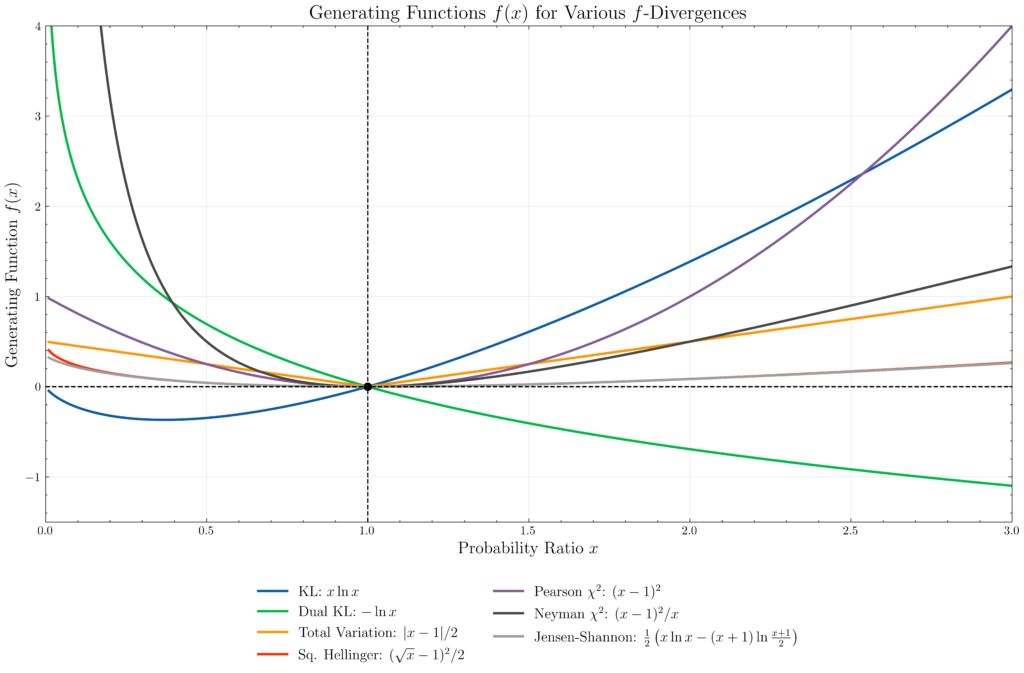
- \(f(x):=x\ln x\) generates the asymmetric Kullback-Leibler (KL) divergence \[D_{\text{KL}}(\boldsymbol{\theta}||\boldsymbol{\theta}’):=\int d\mathbf x p(\mathbf x|\boldsymbol{\theta})\ln\frac{p(\mathbf x|\boldsymbol{\theta})}{p(\mathbf x|\boldsymbol{\theta}’)}\]
- \(f(x):=-\ln x\) generates the dual KL divergence \(D_{\text{KL}}(\boldsymbol{\theta}’||\boldsymbol{\theta})\) (in general, \(D_{xf(1/x)}(\boldsymbol{\theta}||\boldsymbol{\theta}’)=D_{f(x)}(\boldsymbol{\theta}’||\boldsymbol{\theta})\))
- \(f(x):=|x-1|/2\) generates the total variation divergence \[d_{\text{TV}}(\boldsymbol{\theta}||\boldsymbol{\theta}’):=\frac{1}{2}\int d\mathbf x|p(\mathbf x|\boldsymbol{\theta})-p(\mathbf x|\boldsymbol{\theta}’)|\] (indeed, TVD is actually symmetric and obeys the triangle inequality so is a metric in the metric space sense, yet does not admit a Fisher information metric due to the non-differentiability of the absolute value).
- \(f(x):=(\sqrt{x}-1)^2/2\) generates the symmetric squared Hellinger divergence \[d^2_H(\boldsymbol{\theta}||\boldsymbol{\theta}’):=\frac{1}{2}\int d\mathbf x\left(\sqrt{p(\mathbf x|\boldsymbol{\theta})}-\sqrt{p(\mathbf x|\boldsymbol{\theta}’)}\right)^2=1-\int d\mathbf x\sqrt{p(\mathbf x|\boldsymbol{\theta})p(\mathbf x|\boldsymbol{\theta}’)}\]
- \(f(x):=(x-1)^2\) generates the Pearson \(\chi^2\) divergence \[D_{\chi^2}(\boldsymbol{\theta}||\boldsymbol{\theta}’):=\int d\mathbf x\frac{(p(\mathbf x|\boldsymbol{\theta})-p(\mathbf x|\boldsymbol{\theta}’))^2}{p(\mathbf x|\boldsymbol{\theta}’)}\] and \(f(x)=(x-1)^2/x\) generates the dual divergence (called the Neyman \(\chi^2\) divergence) in which one replaces \(p(\mathbf x|\boldsymbol{\theta}’)\mapsto p(\mathbf x|\boldsymbol{\theta})\) in the denominator.
- \(f(x):=\frac{1}{2}\left(x\ln x-(x+1)\ln\frac{x+1}{2}\right)\) generates the symmetric Jensen-Shannon divergence \[d^2_{\text{JS}}(\boldsymbol{\theta}||\boldsymbol{\theta}’):=\frac{D_{\text{KL}}(p_{\boldsymbol{\theta}}||\frac{p_{\boldsymbol{\theta}}+p_{\boldsymbol{\theta}’}}{2})+D_{\text{KL}}(p_{\boldsymbol{\theta}’}||\frac{p_{\boldsymbol{\theta}}+p_{\boldsymbol{\theta}’}}{2})}{2}\]
Problem: What is a fundamental limitation in the family of \(f\)-divergences \(D_f\)? How do integral probability metrics such as the Wasserstein (a.k.a. earth-mover’s) distance address this shortcoming?
Solution:
\[W_{n}(p,p’)=\text{min}_{p(\mathbf x,\mathbf x’)|\int d\mathbf xp(\mathbf x,\mathbf x’)=p(\mathbf x’)\text{ and }\int d\mathbf x’p(\mathbf x,\mathbf x’)=p'(\mathbf x)}\left(\int dp(\mathbf x,\mathbf x’)|\mathbf x-\mathbf x’|^n\right)^{1/n}\]
where the joint probability is \(dp(\mathbf x,\mathbf x’)=d\mathbf xd\mathbf x’p(\mathbf x,\mathbf x’)\).
(include a concrete computation in \(1\) dimension).
Problem: (something about Bregman divergence, comment on how KL div is the only simultaneous f and Bregman divergence)
Solution: