
Problem: Define the signature of a matrix. Hence, state and prove Sylvester’s law of inertia.
Solution: The signature of an \(n\times n\) matrix \(A\) is a \(3\)-tuple \((n_+,n_-,n_0)\) where \(n_+\) is the number of positive eigenvalues of \(A\) (including multiplicity), \(n_-\) is the number of negative eigenvalue of \(A\) (including multiplicity), and \(n_0=\text{dim}\ker A\) is the multiplicity of the zero eigenvalue; thus, \(n_++n_-+n_0=n\).
Let \(A,B\) be real symmetric matrices. Then Sylvester’s law of inertia asserts that \(A\) and \(B\) are congruent matrices iff they have the same signature (which sometimes is called “inertia” because of this invariance under congruence, hence the name).
Proof: It’s easy to see that the nullity \(n_0\) is preserved by congruence transformations. If one can can show that \(n_+\) is also preserved, then it implies \(n_-\) is conserved by virtue of \(n_++n_-+n_0=n\). To show this, the idea is to prove by contradiction, assuming \(n_+\) is not preserved which by dimension counting would imply a non-zero vector living in the intersection of the subspace spanned by the positive-eigenvalue eigenvectors of \(A\) and the congruence-transformed subspace spanned by the non-positive-eigenvalue eigenvectors of \(B\).
Since any real, symmetric matrix \(A\) is isomorphic to a real quadratic form \(Q(\mathbf x):=\mathbf x^TA\mathbf x\), the concepts of signature and Sylvester’s law of inertia can also be reformulated in the language of quadratic forms rather than real symmetric matrices.
Problem: Let \(X\) be a smooth \(n\)-manifold. Explain what it means to place the additional structure of a pseudo-Riemannian metric \(g\) on \(X\). Then explain how Riemannian and Lorentzian geometry are special cases of pseudo-Riemannian geometry.
Solution: A Riemannian metric \(g\) on \(X\) is a type \((0,2)\) tensor field that defines an inner product \(g_x:T_x(X)^2\to\mathbf R\) at the tangent space \(T_x(X)\) of each point \(x\in X\). The “tensor field” part is sometimes rephrased as saying that \(g_x\) is a bilinear form. Moreover, to flesh out the usual axioms of a real inner product space, the Riemannian metric tensor \(g_x\) at each \(x\in X\) must be symmetric \(g_x(v_x,v’_x)=g_x(v’_x,v_x)\) and positive-definite \(v_x\neq 0\Rightarrow g_x(v_x,v_x)>0\).
A pseudo-Riemannian metric relaxes the positive-definite requirement of a Riemannian metric, instead merely requiring non-degeneracy (i.e. at each point \(x\in X\), the zero vector \(0\) is the only vector orthogonal \(g_x(0,v_x)=0\) to all \(v_x\in T_x(X)\)). More concisely, what this is saying is that \(n_0=0\), so the signature of a pseudo-Riemannian metric may be thought of as a pair \((n_+,n_-)\).
Thus, Riemannian metrics are the special subset of pseudo-Riemannian metrics for which \((n_+,n_-)=(n,0)\). Meanwhile, Lorentzian metrics are another special subset of pseudo-Riemannian metrics for which \((n_+,n_-)=(n-1,1)\) (this is the relativists’/ convention). Typically, spacetime \(X\) has dimension \(n=4\), so e.g. the Minkowski metric is said to have signature \((3,1):=(-,+,+,+)\).
Problem: Let \((X,g)\) be a pseudo-Riemannian manifold. Often, one writes the general expression for an infinitesimal line element on \(X\) as \(ds^2=g_{\mu\nu}dx^{\mu}dx^{\nu}\); explain the shorthand being used here.
Solution: This is nothing more than choosing some chart \(x^{\mu}\) on \(X\) and expanding the metric tensor field \(g\) in the coordinate basis \(\{dx^{\mu}\otimes dx^{\nu}\}\) of type \((0,2)\) tensor fields:
\[g=g_{\mu\nu}dx^{\mu}\otimes dx^{\nu}\]
for some real, symmetric scalar fields \(g_{\mu\nu}:X\to\mathbf R\). One then simply writes \(ds^2:=g\) and omits the tensor product \(\otimes\).
Problem: Let \(x(t)\in X\) be a curve on a Riemannian manifold \((X,g)\). By choosing a chart \(x^{\mu}\) to cover a suitable region of \(X\) spanned by the trajectory \(x(t)\), explain how to compute the length \(s\) of the curve \(x(t)\) using the Riemannian metric \(g\).
Solution: Heuristically, it is:
\[s=\int ds=\int\sqrt{g_{\mu\nu}dx^{\mu}dx^{\nu}}=\int dt\sqrt{g_{\mu\nu}(x(t))\dot{x}^{\mu}\dot{x}^{\nu}}\]
Problem: Write down the action \(S\) for a non-relativistic particle of mass \(m\) moving on a Riemannian manifold \((X,g)\). Hence, derive the geodesic equation. What happens if the particle is relativistic?
Solution: A nonrelativistic free particle of mass \(m\) has action \(S=\int dt L\) described by the usual nonrelativistic kinetic Lagrangian:
\[L=\frac{m}{2}|\dot{\mathbf x}|^2\]
The catch is that \(|\dot{\mathbf x}|^2=g_{ij}(\mathbf x)\dot x^{i}\dot x^{j}\) depends on the Riemannian metric \(g\) in which the particle moves. Applying the Euler-Lagrange equations, one finds the equation of motion (called the geodesic equation):
\[\ddot x^i+\Gamma^i_{jk}\dot x^j\dot x^k=0\]
where the Christoffel symbols \(\Gamma^i_{jk}(\mathbf x):=\frac{1}{2}g^{i\ell}(\mathbf x)\left(\frac{\partial g_{\ell j}}{\partial x^k}+\frac{\partial g_{\ell k}}{\partial x^j}-\frac{\partial g_{jk}}{\partial x^{\ell}}\right)\) are analogous to “fictitious forces” on the particle due to the curvature of \(X\).
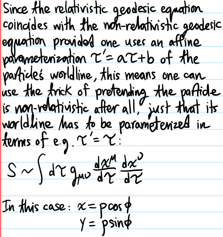
By contrast, a relativistic free particle has action \(S=-mcs=-mc^2\tau\). This can be recast into non-relativistic form \(S=\int dt L\) using the relativistic kinetic Lagrangian:
\[L=-mc\sqrt{g_{\mu\nu}\dot x^{\mu}\dot x^{\nu}}\]
which in flat space \(g_{\mu\nu}=\text{diag}(1,-1,-1,-1)\) reduces to the familiar \(L=-mc^2/\gamma\) (nb. more generally, the quantity under the square root is always \(\geq 0\) for the timelike worldlines of particles). Some comments:
- The stationary action principle \(\delta S=0\) in which the action \(S\) tends to be minimized corresponds to the well-known fact that relativistic free particles travelling in straight line geodesics through spacetime maximize the Minkowski distance \(s\), or equivalently Alice experiences more proper time (i.e. ages more) than Bob in the twin paradox.
- The relativistic action (unlike its non-relativistic counterpart) is manifestly reparameterization invariant.
Now the Euler-Lagrange geodesic equations for the relativistic Lagrangian are almost identical to the non-relativistic case except there’s an additional term:
\[\ddot x^{\mu}+\Gamma^{\mu}_{\nu\rho}(x)\dot x^{\nu}\dot x^{\rho}=\frac{\dot L}{L}\dot x^{\mu}\]
The additional term vanishes \(\dot L=0\) iff \(L=L(\tau’)\) is parameterized as any affine transformation \(s=\tilde{c}\tau+s_0\) of the particle’s proper time \(\tau\) (prove this by showing \(\dot{s}=-\tilde{c}L/mc^2\)). Only in this case does the relativistic geodesic equation reduce to the non-relativistic form:
\[\frac{d^2 x^{\mu}}{ds^2}+\Gamma^{\mu}_{\nu\rho}(x(s))\frac{dx^{\nu}}{ds}\frac{dx^{\rho}}{ds}=0\]
Problem: For \(X=\mathbf R^2\), calculate all non-vanishing Christoffel symbols in the polar coordinate chart \((\rho,\phi)\).
Solution:
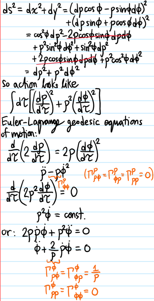
Note it is usually more efficient to compute Christoffel symbols this way rather than using the explicit formula in terms of partial derivatives of the metric \(g\) (though they’re of course equivalent).
Problem: Explain how the presence of a pseudo-Riemannian metric \(g\) on a smooth manifold \(X\) allows one to identify covectors in \(T_x^*(X)\) with tangent vectors in \(T_x(X)\) at each point \(x\in X\).
Solution: Just as in \(X=\mathbf R^n\), one identifies a tangent vector \(\mathbf v\) with its covector \(\mathbf v\cdot\) via the inner product \(\cdot\), so at a given \(x\in X\), one uses the pseudo-inner product \(g_x\) on \(T_x(X)\) to make the exact same identification \(v_x\leftrightarrow g_x(v_x,\space)\) (this sometimes called the musical isomorphism induced by \(g\) in light of the map \(\flat_x:T_x(X)\to T^*_x(X)\) defined by \(v_x^{\flat_x}(v’_x):=g(v_x,v’_x)\) and its inverse \(\sharp_x=\flat_x^{-1}\)).
In some chart \(x^{\mu}\), one can write the \(1\)-form \(v^{\flat}=(v^{\flat})_{\mu}dx^{\mu}\) with components \((v^{\flat})_{\mu}=v^{\flat}(\partial_{\mu})=g(v,\partial_{\mu})=g_{\mu\nu}v^{\nu}\) where \(v^{\nu}=v(x^{\nu})\) are the components of its musically isomorphic vector field \(v=v^{\nu}\partial_{\nu}\) in the same coordinate basis. Physicists typically abuse notation by merely writing \((v^{\flat})_{\mu}=g_{\mu\nu}v^{\nu}\) as just \(v_{\mu}=g_{\mu\nu}v^{\nu}\), identifying \(v^{\flat}\equiv v\) under the musical isomorphism. But then this lazy notation makes it look as if the metric \(g\) performs a trivial mechanical action of just “lowering the index” on \(v\).
Problem: Define a tensor field \(g^*\) that performs the trivial mechanical action of “raising the index” on a \(1\)-form \(A\).
Solution: Define \(g^*_x:T^*_x(X)^2\to\mathbf R\) to be a type \((2,0)\) tensor given by:
\[g^*(A,A’):=g(A^{\sharp}, A’^{\sharp})\]
Then on the one hand, in some chart \(x^{\mu}\), one has:
\[g^*(v^{\flat},v’^{\flat})=g(v,v’)=g_{\mu\nu}v^{\mu}v’^{\nu}\]
On the other hand, in that same chart \(x^{\mu}\), one has:
\[g^*(v^{\flat},v’^{\flat})=(g^*)^{\mu\nu}(v^{\flat})_{\mu}(v’^{\flat})_{\nu}=(g^*)^{\mu\nu}g_{\mu\rho}v^{\rho}g_{\nu\sigma}v’^{\sigma}=(g^*)^{\rho\sigma}g_{\mu\rho}g_{\nu\sigma}v^{\mu}v’^{\nu}\]
This implies \(g_{\mu\nu}=(g^*)^{\rho\sigma}g_{\mu\rho}g_{\nu\sigma}\). Since \(g\) is non-degenerate (the \(N_0=0\) axiom of a pseudo-Riemannian metric), it follows that \(\det g_{\mu\nu}\neq 0\) is invertible, so the only possibility is \((g^*)^{\mu\nu}g_{\nu\rho}=\delta^{\mu}_{\rho}\), i.e. \(g^*\sim g^{-1}\). It is common practice to just drop the \(*\) and write \(g^{\mu\nu}\) in lieu of \((g^*)^{\mu\nu}\). With this lazy notation, \(g^{\mu\nu}\) looks like it just “raises the index” on \(A^{\mu}=g^{\mu\nu}A_{\nu}\) (where one last abuse of notation \((A^{\sharp})^{\mu}=A^{\mu}\) has been made!). cf. raising lowering operators \(a,a^{\dagger}\) in quantum mechanics.
Problem: What is the canonical volume form on a smooth, orientable pseudo-Riemannian \(n\)-manifold \((X,g)\)? Why is it canonical?
Solution: In a chart \(x^{\mu}\) in which the pseudo-Riemannian metric has components \(g=g_{\mu\nu}dx^{\mu}\otimes dx^{\nu}\), the canonical volume form is \(\sqrt{|\det g|}dx^1\wedge…\wedge dx^n\). This is indeed a volume form because it is a top form with \(\det g\neq 0\) nowhere vanishing for same reasons as before. Moreover, it is canonical because, despite appearances, it does not depend on the choice of chart \(x^{\mu}\) (provided it’s the same orientation) as \(\sqrt{|\det g|}\) is a scalar density of weight \(1\) whereas \(dx^1\wedge…\wedge dx^n\) is a scalar density of weight \(-1\).
Problem: Let \((X,g)\) be a smooth, \(n\)-dimensional, orientable pseudo-Riemannian manifold, and let \(\omega\in\Omega^k(X)\) be a differential \(k\)-form on \(X\). Define the Hodge dual \((n-k)\)-form \(\star\omega\in\Omega^{n-k}(X)\) on \(X\).
Solution: The Hodge dual \(\star\omega\in\Omega^{n-k}(X)\) is defined to be the unique differential \((n-k)\)-form such that for all test differential \(k\)-forms \(\omega’\in\Omega^k(X)\) one has the equality of top forms:
\[\omega’\wedge\star\omega=\widetilde{\langle\omega’,\omega\rangle}\sqrt{|\det g|}dx^1\wedge…\wedge dx^n\]
Here, the operation \(\widetilde{\langle\omega’,\omega\rangle}\) is defined for \(\omega’=A’_1\wedge…\wedge A’_k\) and \(\omega=A_1\wedge…\wedge A_k\) by the Gram determinant:
\[\widetilde{\langle\omega’,\omega\rangle}:=\det\begin{pmatrix}g^*(A’_1,A_1) & \dots & g^*(A’_1,A_k) \\ \vdots & \ddots & \vdots \\ g^*(A’_k,A_1) & \dots & g^*(A’_k,A_k)\end{pmatrix}\]
and extended to arbitrary differential \(k\)-forms \(\omega’,\omega\in\Omega^k(X)\) by bilinearity. It is easy to check that the Hodge star \(\star:\Omega^k(X)\to\Omega^{n-k}(X)\) is a linear transformation \(\star(\phi_1\omega_1+\phi_2\omega_2)=\phi_1\star\omega_1+\phi_2\star\omega_2\) between \(2\) vector spaces of the same dimension \(\dim\Omega^k(X)={n\choose k}={n\choose n-k}=\dim\Omega^{n-k}(X)\). Moreover, it is either an involution or behaves like multiplication by \(i\) in the sense that \(\star^2=(-1)^{k(n-k)+n_-}\).
Problem: For flat Minkowski spacetime \(X=\mathbf R^{1+3}\) with the Lorentzian metric \(ds^2=c^2dt^2-dx^2-dy^2-dz^2\) and orientation defined by the canonical volume form \(cdt\wedge dx\wedge dy\wedge dz\), compute the Hodge dual:
\[\star(e^{-x\cos y}dy\wedge dt+4tz^2 dx\wedge dz)\]
Solution: By linearity, one can focus on computing Hodge duals of the basis \(2\)-forms \(\star (dy\wedge dt)\) and \(\star(dx\wedge dz)\). Demonstrating this for \(\star (dy\wedge dt)\), the idea is to (roughly speaking) wedge it against itself and exploit the defining property of the Hodge dual:
\[dy\wedge dt\wedge\star(dy\wedge dt)=\det\begin{pmatrix}g^{yy} & g^{yt} \\ g^{ty} & g^{tt}\end{pmatrix}cdt\wedge dx\wedge dy\wedge dz\]
\[=\det\begin{pmatrix}-1 & 0 \\ 0 & 1/c^2\end{pmatrix}cdt\wedge dx\wedge dy\wedge dz\]
\[=-\frac{1}{c}dt\wedge dx\wedge dy\wedge dz\]
\[=-\frac{1}{c}dy\wedge dt\wedge dx\wedge dz\]
In this case, one can directly read off the answer \(\star(dy\wedge dt)=-c^{-1}dx\wedge dz\) or equivalently \(\star(dy\wedge dct)=dz\wedge dx\). Analogously, one can check \(\star(dx\wedge dz)=dy\wedge dct\) (consistent with the earlier identity for \(\star^2\)), so the final answer is:
\[\star(e^{-x\cos y}dy\wedge dt+4tz^2 dx\wedge dz)=\frac{e^{-x\cos y}}{c}dz\wedge dx+4tz^2dy\wedge dct\]
For more general non-orthogonal metrics \(g\), one cannot simply read off the answer like that but should set up an ansatz for the Hodge dual like \(\star(dy\wedge dt)=c_{tx}dt\wedge dx+c_{ty}dt\wedge dy+c_{tz}dt\wedge dz+c_{xy}dx\wedge dy+c_{xz}dx\wedge dz+c_{yz}dy\wedge dz\) and obtaining the coefficients by wedging against the relevant basis differential forms.
Problem: Let \((X,g)\) be a smooth, \(n\)-dimensional pseudo-Riemannian manifold. Just as the metric tensor field \(g\) induces a pseudo-inner product between tangent vectors at each point across the manifold \(X\), show that \(g\) also induces an inner product on the space \(\Omega^k(X)\) of differential \(k\)-forms on \(X\).
Solution: Given \(2\) differential \(k\)-forms \(\omega,\omega’\in\Omega^k(X)\), their \(g\)-induced inner product is defined by:
\[\langle\omega,\omega’\rangle:=\int_{X}\omega\wedge\star\omega’\]
(this is well-defined because \(\omega\wedge\star\omega’\in\Omega^n(X)\) is indeed a top form as observed earlier).
Problem: Having endowed \(\Omega^k(X)\) with an inner product, one can define the adjoint (sometimes called the codifferential) \(d^{\dagger}:\Omega^k(X)\to\Omega^{k-1}(X)\) of the exterior derivative operator \(d:\Omega^{k-1}(X)\to\Omega^k(X)\) by insisting that for arbitrary differential forms \(\omega\in\Omega^{k-1}(X),\omega’\in\Omega^k(X)\):
\[\langle d\omega,\omega’\rangle=\langle\omega,d^{\dagger}\omega’\rangle\]
(the LHS is the inner product on \(\Omega^k(X)\) whereas the RHS is the inner product on \(\Omega^{k-1}(X)\)). Show that if the underlying pseudo-Riemannian manifold \(X\) is closed, then:
\[d^{\dagger}=(-1)^{n(k+1)+1+n_-}\star d\space\star\]
Solution: Applying graded integration by parts and Stokes’ theorem:
\[\langle d\omega,\omega’\rangle=\int_{\partial X}\omega\wedge\star\omega’+(-1)^k\int_X\omega\wedge d\star\omega’\]
The first term vanishes because \(X\) is assumed to be closed, and by comparing with the expected form:
\[\langle\omega,d^{\dagger}\omega’\rangle=\int_X\omega\wedge\star d^{\dagger}\omega’\]
it is clear this would hold provided:
\[(-1)^kd\star=\star d^{\dagger}\]
Isolating for \(d^{\dagger}\) by acting with \(\star\) on both sides, using \(\star^2=(-1)^{(k-1)(n-k+1)+n_-}\), and exploiting trivial identities like \((-1)^{k^2-k}=1\) and \((-1)^{-n}=(-1)^n\) for \(k,n\in\mathbf Z\) leads to the claimed result.
Problem: Using the technology of \(d^{\dagger}\), define the Laplace-de Rham operator \(\Delta:\Omega^k(X)\to\Omega^k(X)\). For the case of a scalar field \(k=0\), show that the action of the Laplace-de Rham operator \(\Delta\) coincides with that of the negative Laplacian \(-\nabla^2\) (sometimes called the Laplace-Beltrami operator).
Solution: One has the positive semi-definite Laplace-de Rham operator:
\[\Delta:=(d+d^{\dagger})^2=\{d,d^{\dagger}\}\]
thanks to nilpotence \(d^2=(d^{\dagger})^2=0\). For a scalar field \(\phi\in C^{\infty}(X)\), \(d^{\dagger}\phi=0\) so:
\[\Delta\phi=d^{\dagger}d\phi=(-1)^{n_-+1}\star d(\partial_{\mu}\phi\star dx^{\mu})\]
The Hodge dual of the \(\mu^{\text{th}}\) basis \(1\)-form can be checked to be:
\[\star dx^{\mu}=(-1)^{\nu}g^{\mu\nu}\sqrt{|\det g|}dx^0\wedge…\wedge dx^{\nu-1}\wedge dx^{\nu+1}\wedge…\wedge dx^{n-1}\]
Thus:
\[d(\partial_{\mu}\phi\star dx^{\mu})=\partial_{\nu}\left(\sqrt{|\det g|}g^{\mu\nu}\partial_{\mu}\phi\right)dx^0\wedge…\wedge dx^{n-1}\]
And finally, the Hodge dual of a top form returns a scalar field:
\[\star (dx^0\wedge…\wedge dx^{n-1})=\frac{\sqrt{|\det g|}}{\det g}=\frac{(-1)^{n_-}}{\sqrt{|\det g|}}\]
Thus, one obtains:
\[\Delta\phi=-\frac{1}{\sqrt{|\det g|}}\partial_{\nu}\left(\sqrt{|\det g|}g^{\mu\nu}\partial_{\mu}\phi\right)=-\nabla^2\phi\]
Problem: Let \(\omega\in\Omega^k(X)\) be a differential \(k\)-form on a closed, Riemannian manifold \((X,g)\). Explain what it means for \(\omega\) to be harmonic. Furthermore, prove that \(\omega\) is harmonic iff it is both closed \(d\omega=0\) and co-closed \(d^{\dagger}\omega=0\) (this equivalence underlies the Hodge decomposition theorem and hence the rest of Hodge theory).
Solution: This is just a generalization of the usual notion of a harmonic scalar field obeying Laplace’s equation \(\nabla^2\phi=0\), only now the Laplacian \(\nabla^2\) is replaced by the Laplace-de Rham operator \(\Delta\) and the scalar field \(\phi\) by an arbitrary differential \(k\)-form \(\omega\in\Omega^k(X)\):
\[\Delta\omega=0\]
Because \(X\) is closed, one can say:
\[\langle\omega,\Delta\omega\rangle=\langle\omega, dd^{\dagger}\omega\rangle+\langle\omega,d^{\dagger}d\omega\rangle\]
\[=\langle d^{\dagger}\omega,d^{\dagger}\omega\rangle+\langle d\omega,d\omega\rangle\]
If \(\Delta\omega=0\) is harmonic, then it follows \(\langle d^{\dagger}\omega,d^{\dagger}\omega\rangle=\langle d\omega,d\omega\rangle=0\) because \(g\) is Riemannian, so in particular \(d\omega=d^{\dagger}\omega=0\). The converse is trivial: \(\Delta\omega=dd^{\dagger}\omega+d^{\dagger}d\omega=d0+d^{\dagger}0=0\).
Problem: Let \(X\) be a smooth manifold not necessarily equipped with a metric \(g\). What does it mean to endow \(X\) with the structure of a affine connection \(\nabla\)?
Solution: An affine connection is any map \(\nabla:\mathfrak{X}(X)^2\to\mathfrak{X}(X)\) which is linear in its first tangent vector field argument but acts like a tangent vector (more precisely, like a derivation) in its second tangent vector field argument. Thus, \(\nabla\) is not tensorial because it is not linear in that second argument. Nevertheless, given a (possibly non-coordinate) basis \(\text{span}_{\mathbf R}\{e_{\mu}\}=\mathfrak{X}(X)\) of tangent vector fields, one can still define affine connection coefficients for \(\nabla\):
\[\nabla_{\nu}e_{\rho}=\Gamma^{\mu}_{\nu\rho}e_{\mu}\]
with \(\nabla_{\nu}:=\nabla_{e_{\nu}}\) a shorthand. The map \(\nabla_v:\mathfrak{X}(X)\to\mathfrak{X}(X)\) for some fixed tangent vector field \(v\in\mathfrak{X}(X)\) is called the covariant derivative along \(v\).
Problem: Let \(X\) be a smooth manifold. For two tangent vector fields \(v,v’\in\mathfrak{X}(X)\), given a (possibly non-coordinate) basis \(\text{span}_{\mathbf R}\{e_{\mu}\}=\mathfrak{X}(X)\) of tangent vector fields so that \(v=v^{\mu}e_{\mu}\) and \(v’=v’^{\nu}e_{\nu}\), show that:
\[\nabla_vv’=v^{\nu}(e_{\nu}(v’^{\mu})+\Gamma^{\mu}_{\nu\rho}v’^{\rho})e_{\mu}=v^{\nu}\nabla_{\nu}v’\]
Solution: This is a straightforward application of the properties of affine connections. The only thing to watch out for is that the affine connection is extended to act on scalar fields \(\phi\in C^{\infty}(X)\) in the obvious way:
\[\nabla_v\phi:=v(\phi)=\mathcal L_v\phi\]
In particular, \(\nabla_{\mu}\phi=e_{\mu}(\phi)\), and if \(e_{\mu}=\partial_{\mu}\) happens to be a coordinate basis for \(\mathfrak{X}(X)\), then the covariant derivative \(\nabla_{\mu}=\partial_{\mu}\) coincides with the partial derivative on scalar fields.
Problem: For tangent vector fields \(v,v’\in\mathfrak{X}(X)\), compare the covariant derivative \(\nabla_vv’\) with the Lie derivative \(\mathcal L_vv’\) (both of which are tangent vector fields).
Solution: Basically, in the case of the Lie derivative \(\mathcal L_vv’=[v,v’]\), both entries of the commutator are subject to the product rule, for example \([vv^{\prime\prime},v’]=v[v^{\prime\prime},v’]+[v,v’]v^{\prime\prime}\), so in particular are nonlinear (being additive but inhomogeneous). By contrast, in the covariant derivative \(\nabla_vv’\), the \(v\)-argument is explicitly made to be linear (though the \(v’\) argument behaves in the same way as both arguments of the Lie derivative), so this is what allows familiar linear algebraic expressions like \(\nabla_v=v^{\mu}\nabla_{\mu}\) to be written (this was proven above in the form \(\nabla_vv’=v^{\nu}\nabla_{\nu}v’\)).
Problem: Explain how to compute the covariant derivative of a \(1\)-form \(A\in\Omega^1(X)\) along a tangent vector field \(v\in\mathfrak{X}(X)\) to end up with another \(1\)-form \(\nabla_v A\).
Solution: As a \(1\)-form, \(A\) maps a tangent vector field \(v’\in\mathfrak{X}(X)\) to a scalar field \(A(v’)\in C^{\infty}(X)\). But earlier, it was already explained one can take the covariant derivative of a scalar field, so it makes sense to compute \(\nabla_v(A(v’))=v(A(v’))\). However, by insisting that the product rule holds in the sense:
\[\nabla_v(A(v’))=(\nabla_vA)(v’)+A(\nabla_vv’)\]
So the desired definition ought to be:
\[(\nabla_vA)(v’):=v(A(v’))-A(\nabla_vv’)\]
or in a basis of \(\mathfrak{X}(X)\):
\[(\nabla_vA)(v’)=(\nabla_{\mu}A)_{\nu}v^{\mu}v’^{\nu}\]
with \((\nabla_{\mu}A)_{\nu}=\partial_{\mu}A_{\nu}-\Gamma^{\rho}_{\mu\nu}A_{\rho}\).
(note: it is possible to generalize the action of the covariant derivative \(\nabla_v\) to arbitrary tensor fields, but this construction is omitted here).
Problem: Let \(X\) be a smooth manifold equipped with an affine connection \(\nabla\). What does it mean for a tangent vector field \(v’\in\mathfrak{X}(X)\) to be parallel transported along another tangent vector field \(v\in\mathfrak{X}(X)\)?
Solution: It means that \(\nabla_{v}v’=0\). In a coordinate basis \(\{\partial_{\mu}\}\) of tangent vector fields, this is equivalent to (using the chain rule \(\frac{dv'(x(\tau))}{d\tau}=\frac{dx^{\mu}}{d\tau}\frac{\partial v’}{\partial x^{\mu}}=v^{\mu}\partial_{\mu}v’\)):
\[\frac{dv’^{\mu}}{d\tau}+\Gamma^{\mu}_{\nu\rho}v^{\nu}v’^{\rho}=0\]
which in particular reduces to the geodesic equation when \(v’=v\) (thus, geodesics are nothing more than the integral curves that arise from parallel transporting a tangent vector field along itself).
Problem: Let \(X\) be a smooth manifold equipped with an affine connection \(\nabla\). Define the type-\((1,2)\) torsion tensor field \(T\) of \(\nabla\), and compute the components of \(T\) in a coordinate basis.
Solution: For a \(1\)-form \(A\in\Omega^1(X)\) and tangent vector fields \(v,v’\in\mathfrak{X}(X)\), one has:
\[T(A,v,v’):=A(\nabla_vv’-\nabla_{v’}v-[v,v’])\]
One should check that \(T\) is indeed a tensor, since the affine connection \(\nabla\) is not a tensor as mentioned earlier. It is easy to see that \(T\) is linear in \(A\), and it is linear in \(v\) iff it is linear in \(v’\) because of antisymmetry \(T(A,v’,v)=-T(A,v,v’)\). Furthermore, it is easy to see that \(T(A,v_1+v_2,v’)=T(A,v_1,v’)+T(A,v_2,v’)\). The tricky property to prove is that \(T(A,\phi v,v’)=\phi T(A,v,v’)\) for any scalar field \(\phi\in C^{\infty}(X)\) (it must be a scalar field and not just some scalar \(\phi\in\mathbf R\) because one is trying to show that \(T\) is a tensor field not just a tensor):
\[T(A,\phi v,v’)=A(\nabla_{\phi v}v’-\nabla_{v’}(\phi v)-[\phi v,v’])\]
\[=A(\phi\nabla_vv’-v'(\phi)v-\phi\nabla_{v’}v-\phi[v,v’]+v'(\phi)v)\]
\[=A(\phi\nabla_vv’-\phi\nabla_{v’}v-\phi[v,v’])\]
\[=\phi A(\nabla_vv’-\nabla_{v’}v-[v,v’])=\phi T(A,v,v’)\]
Thus, in a coordinate basis \(\{\partial_{\mu}\}\) of \(\mathfrak{X}(X)\), the components \(T^{\rho}_{\mu\nu}:=T(dx^{\rho},\partial_{\mu},\partial_{\nu})\) are tensorial:
\[T^{\rho}_{\mu\nu}=\Gamma^{\rho}_{\mu\nu}-\Gamma^{\rho}_{\nu\mu}\]
where Clairaut’s theorem \([\partial_{\mu},\partial_{\nu}]=0\) for a coordinate basis has been used.
Problem: Let \(X\) be a smooth manifold equipped with an affine connection \(\nabla\). Define the type-\((1,3)\) Riemann curvature tensor field \(R\) of \(\nabla\), and compute the components of \(R\) in a coordinate basis.
Solution: For a \(1\)-form \(A\in\Omega^1(X)\) and tangent vector fields \(v,v’,v^{\prime\prime}\in\mathfrak{X}(X)\), one has:
\[R(A,v,v’,v^{\prime\prime}):=A(\nabla_v\nabla_{v’}v^{\prime\prime}-\nabla_{v’}\nabla_vv^{\prime\prime}-\nabla_{[v,v’]}v^{\prime\prime})\]
Similar to the torsion tensor field \(T\), one should check that \(R\) genuinely deserves its designation as a tensor field. In a coordinate basis \(\{\partial_{\mu}\}\) of \(\mathfrak{X}(X)\), the (slightly awkward but conventional) tensor components \(R^{\sigma}_{\rho\mu\nu}:=R(dx^{\sigma},\partial_{\mu},\partial_{\nu},\partial_{\rho})\) are:
\[R^{\sigma}_{\rho\mu\nu}=\partial_{\mu}\Gamma^{\sigma}_{\nu\rho}-\partial_{\nu}\Gamma^{\sigma}_{\mu\rho}+\Gamma^{\lambda}_{\nu\rho}\Gamma^{\sigma}_{\mu\lambda}-\Gamma^{\lambda}_{\mu\rho}\Gamma^{\sigma}_{\nu\lambda}\]
where again Clairaut’s theorem \([\partial_{\mu},\partial_{\nu}]=0\) for a coordinate basis has been used. Again similar to the case for \(T\), the antisymmetry \(R(A,v’,v,v^{\prime\prime})=-R(A,v,v’,v^{\prime\prime})\) manifests at the component level as \(R^{\sigma}_{\rho\nu\mu}=-R^{\sigma}_{\rho\mu\nu}\).
Problem: (about the Ricci identity connecting \(T\) and \(R\) together in terms of the commutator of covariant derivatives)
Solution:
Problem: State and prove the fundamental theorem of pseudo-Riemannian geometry.
Solution: Let \((X,g)\) be a smooth, pseudo-Riemannian manifold. Then there exists a unique affine connection \(\nabla\) (called the Levi-Civita connection) which is torsion-free \(T=0\) and \(g\)-compatible in the sense that \(\nabla_v g=0\) for all tangent vector fields \(v\in\mathfrak{X}(X)\).
Proof: (need to go back up and define covariant differentiation of a tensor field).
Problem: Let \(X\) be a pseudo-Riemannian manifold thus equipped with the Levi-Civita connection \(\nabla\). Explain how to obtain the geodesic deviation equation (“tidal acceleration equation“):
\[\frac{D^2 J^{\mu}}{D\tau^2}=R^{\mu}_{\nu\rho\sigma}v^{\nu}v^{\rho}J^{\sigma}\]
for the Jacobi tangent vector field \(J\) of a family of affinely-parameterized geodesics.
Solution: For each value of a real parameter \(\varphi\in\mathbf R\) (e.g. rapidity), let \(x(\tau;\varphi)\in X\) be a geodesic (which could be timelike, spacelike or null) in \(X\) affinely parameterized by some \(\tau\in\mathbf R\) (e.g. proper time). From this, one can then construct the \(2\) tangent vector fields:
\[v:=\frac{\partial x}{\partial\tau}\]
\[J:=\frac{\partial x}{\partial\varphi}\]
The first lemma one needs to check is that \(\mathcal L_vJ=[v,J]=0\). This follows from working in a coordinate basis:
\[[v,J]^{\mu}=v^{\nu}\partial_{\nu}J^{\mu}-J^{\nu}\partial_{\nu}v^{\mu}\]
and using the chain rule to write \(\frac{\partial x^{\nu}}{\partial\tau}\frac{\partial J^{\mu}}{\partial x^{\nu}}=\frac{\partial J^{\mu}}{\partial\tau}\) and \(\frac{\partial x^{\nu}}{\partial\varphi}\frac{\partial v^{\mu}}{\partial x^{\nu}}=\frac{\partial v^{\mu}}{\partial\varphi}\). so that by Clairaut’s theorem:
\[[v,J]^{\mu}=\frac{\partial J^{\mu}}{\partial\tau}-\frac{\partial v^{\mu}}{\partial\varphi}=\frac{\partial^2 x^{\mu}}{\partial \varphi\partial\tau}-\frac{\partial^2 x^{\mu}}{\partial \tau\partial\varphi}=0\]
Since the Levi-Civita connection is torsion-free \(T=0\), this implies \(\nabla_vJ=\nabla_Jv\). Recalling that \(\nabla_vv=0\) is tangent to the geodesics, the Riemann curvature tensor field is thus:
\[R(v,J)v=\nabla_v\nabla_Jv-\nabla_J\nabla_vv-\nabla_{[v,J]}v=\nabla_v\nabla_vJ\]
which leads to the desired result in the coordinate basis after writing the “material derivative” \(D/D\tau:=\nabla_v\) along the geodesic.
Problem: Let \(X\) be a smooth manifold equipped with a torsion-free \(T=0\) affine connection \(\nabla\). Show that the components \(R_{\sigma\rho\mu\nu}:=g_{\sigma\lambda}R^{\lambda}_{\rho\mu\nu}\) of the Riemann curvature tensor field obey the first and second Bianchi identities:
\[R(v,v’)v^{\prime\prime}+R(v’,v^{\prime\prime})v+R(v^{\prime\prime},v)v’=0\Leftrightarrow R_{\sigma[\rho\mu\nu]}=0\]
\[\nabla_vR(v’,v^{\prime\prime})v^{\prime\prime\prime}+\nabla_{v’}R(v,v^{\prime\prime},v)v^{\prime\prime\prime}+\nabla_{v^{\prime\prime}}R(v,v’)v^{\prime\prime\prime}=0\Leftrightarrow \nabla_{[\lambda}R_{\sigma\rho]\mu\nu}=0\]
If \(X\) is furthermore a pseudo-Riemannian manifold so that \(\nabla\) is the Levi-Civita connection, show that:
\[R_{\sigma\rho\mu\nu}=R_{\mu\nu\sigma\rho}=-R_{\rho\sigma\mu\nu}=-R_{\sigma\rho\nu\mu}\]
(due to these various symmetries, it turns out in dimension \(d\), the Riemann curvature tensor field has \(d^2(d^2-1)/12\) independent components which for \(d=4\) is \(20\) components).
Solution: Work in Riemann normal coordinates (the first Bianchi identity simply expresses the “boundary of a boundary is zero” idea while the second Bianchi identity is just the Jacobi identity).
Problem: Construct the Ricci tensor field \(R_{\mu\nu}(x)\) and the Ricci scalar field \(R(x)\) in terms of the components of the Riemann curvature tensor field \(R^{\rho}_{\mu\rho\nu}(x)\) in some chart for a pseudo-Riemannian manifold \((X,g)\). Hence, define the Einstein tensor field \(G_{\mu\nu}(x)\) and show that it is symmetric \(G_{\nu\mu}=G_{\mu\nu}\) and divergence-free \(\nabla^{\mu}G_{\mu\nu}=0\).
Solution: One has:
\[R_{\mu\nu}:=R^{\rho}_{\mu\rho\nu}\]
\[R:=g^{\mu\nu}R_{\mu\nu}=R^{\mu}_{\mu}\]
\[G_{\mu\nu}:=R_{\mu\nu}-\frac{1}{2}Rg_{\mu\nu}\]
To show that \(G_{\mu\nu}\) is symmetric, it suffices to note that both \(R_{\mu\nu}\) and \(g_{\mu\nu}\) are symmetric. To show \(G_{\mu\nu}\) is divergence free, one has to contract the \(2^{\text{nd}}\) Bianchi identity twice to obtain the contracted Bianchi identity \(\nabla^{\mu}R_{\mu\nu}=\frac{1}{2}\nabla_{\nu}R\).
Problem: Hence, state the Einstein field equations for the \(d(d+1)/2=10\) components of the metric tensor field of pseudo-Riemannian spacetime. Show that in the Newtonian limit they reduce to Poisson’s equation \(\biggr|\frac{\partial}{\partial\mathbf x}\biggr|^2\phi=4\pi G\rho\) for the Newtonian gravitational potential \(\phi(\mathbf x)\).
Solution: First, one has to be clear about what it means to take the “Newtonian limit”. This means \(3\) conditions:
- Nonrelativistic speeds \(|v^i|\ll |v^0|\)
- Weak gravitational field \(g\approx\eta\) (and I guess \(\Lambda=0\)…)
- Static gravitational field \(\partial_0g=0\)
With these conditions, it is possible to start from the geodesic equation, and arrive at Newton’s second law \(\ddot{\mathbf x}=-\frac{\partial\phi}{\partial\mathbf x}\) provided one makes the key identification \(g_{00}=1+\frac{2\phi}{c^2}\). Substituting this into the trace-reversed form of the EFE:
\[R_{\mu\nu}=\frac{8\pi G}{c^4}\left(T_{\mu\nu}-\frac{1}{2}Tg_{\mu\nu}\right)\]
one can show that it reduces to Poisson’s equation in the Newtonian limit again.