
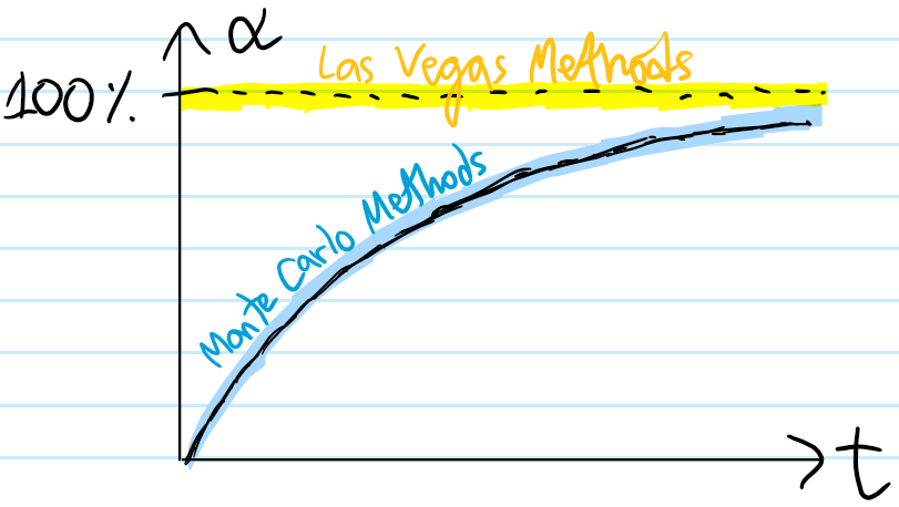
Problem: Distinguish between Las Vegas methods and Monte Carlo methods.
Solution: Both are umbrella terms referring to broad classes of methods that draw (repeatedly) from (not necessarily i.i.d.) random variables to compute the value of some deterministic variable. Here, “compute” means “find that deterministic value with certainty” in the case of a Las Vegas method whereas “compute” means “(point) estimate” in the case of a Monte Carlo method. Thus, their key difference lies in how they tradeoff time \(t\) vs. accuracy \(\alpha\):
Problem: Given a scalar continuous random variable with probability density function \(p(x)\), how can one sample faithfully from such an \(x\sim p(x)\)?
Solution: Fundamentally, a computer can (approximately) draw from a uniform random variable \(u\in [0,1]\) (using seed-based pseudorandom number generators for instance). In order to convert this \(u\to x\), the standard way is to use the cumulative distribution function of \(x\):
\[\int_{-\infty}^xdx’p(x’):=u\]
Then, as the probability density of \(u\) is uniform \(p(u)=1\), the probability density of \(x\) will be \(p(x)=\frac{du}{dx}p(u)\). As the CDF is a monotonically increasing bijection, there always exists an \(x=x(u)\) for each \(u\in[0,1]\). And intuitively, this whole sampling scheme should make a lot of sense:

Problem: So, it seems like the above “inverse CDF trick” has solved the problem of sampling from an arbitrary random variable \(x\) (and it generalizes to the case of a higher-dimensional random vector \(\mathbf x\in\mathbf R^n\) by sampling conditionally). So how come in many practical applications this “sampling” problem can still be difficult?
Solution: In practice, one may not have access to \(p(\mathbf x)\) itself, but only the general shape \(\tilde p(\mathbf x)=Zp(\mathbf x)\) of it (e.g. in Bayesian inference). One might object that \(Z\) is known, namely \(Z=\int d^n\mathbf x\tilde p(\mathbf x)\) can be written explicitly as an \(n\)-dimensional integral, so wherein lies the difficulty? The difficulty lies in evaluating the integral, which suffers from the curse of dimensionality if \(n\gg 1\) is large (just imagine approximating the integral by a sum, and then realizing that the number of terms \(N\) in such a series would grow as \(N\sim O(\exp n)\)). The inverse CDF trick thus fails because it requires one to have \(p(\mathbf x)\) itself, not merely \(\tilde p(\mathbf x)\).
Problem: Describe the Monte Carlo method known as importance sampling for estimating the expectation \(\langle f(\mathbf x)\rangle\) of a random variable \(f(\mathbf x)\).
Solution: Importance sampling consists of a deliberate reframing of the integrand of the expectation inner product integral:
\[\langle f(\mathbf x)\rangle=\int d^n\mathbf x p(\mathbf x)f(\mathbf x)=\int d^n\mathbf x q(\mathbf x)\frac{p(\mathbf x)f(\mathbf x)}{q(\mathbf x)}\]
in other words, replacing \(p(\mathbf x)\mapsto q(\mathbf x)\) and \(f(\mathbf x)\mapsto p(\mathbf x)f(\mathbf x)/q(\mathbf x)\). There are \(2\) cases in which importance sampling can be useful. The first case is related to the previous problem, namely when sampling directly from \(p(\mathbf x)\) is too difficult, in which case \(q(\mathbf x)\) should be chosen to be easier to both sample from and evaluate than \(p(\mathbf x)\). The second case is, even if sampling directly from \(p(\mathbf x)\) is feasible, it can still be useful to instead sample from \(q(\mathbf x)\) as a means of reducing the variance of the Monte Carlo estimator. That is, whereas the original Monte Carlo estimator of the expectation involving \(N\) i.i.d. draws \(\mathbf x_1,…,\mathbf x_N\) from \(p(\mathbf x)\) is \(\sum_{i=1}^Nf(\mathbf x_i)/N\) with variance \(\sigma^2_{f(\mathbf x)}/N\), the new Monte Carlo estimator of the expectation involving \(N\) i.i.d. draws from \(q(\mathbf x)\) is \(\sum_{i=1}^Np(\mathbf x_i)f(\mathbf x_i)/q(\mathbf x_i)N\) with variance \(\sigma^2_{p(\mathbf x)f(\mathbf x)/q(\mathbf x)}/N\); for importance sampling to be useful, \(q(\mathbf x)\) should be chosen such that:
\[\sigma^2_{p(\mathbf x)f(\mathbf x)/q(\mathbf x)}<\sigma^2_{f(\mathbf x)}\]
One can explicitly find the function \(q(\mathbf x)\) that minimizes the variance functional of \(q(\mathbf x)\) (using a Lagrange multiplier to enforce normalization \(\int d^n\mathbf x q(\mathbf x)=1\)):
\[q(\mathbf x)\sim p(\mathbf x)|f(\mathbf x)|\]
In and of itself, this \(q(\mathbf x)\) cannot be used because it contains the difficult piece \(p(\mathbf x)\). Nevertheless, motivated by this result, one can heuristically importance sample using a \(q(\mathbf x)\) which ideally is large at \(\mathbf x\in\mathbf R^n\) where \(p(\mathbf x)|f(\mathbf x)|\) is large. Intuitively, this is because that’s the integrand in the expectation inner product integral, so locations where it’s large will contribute most to the integral, hence are the most “important” regions to sample from with \(q(\mathbf x)\).
One glaring flaw with the above discussion is that if \(Z\) is not known, then it will also be impossible to sample from \(p(\mathbf x)\). Instead, suppose as before that only the shape \(\tilde p(\mathbf x)=Zp(\mathbf x)\) is known with \(Z=\int d^n\mathbf x\tilde p(\mathbf x)\). Thus, the expectation is:
\[\frac{\int d^n\mathbf x\tilde{p}(\mathbf x)f(\mathbf x)}{\int d^n\mathbf x\tilde{p}(\mathbf x)}\]
The key is to notice that the denominator is just the \(f(\mathbf x)=1\) special case of the numerator, hence the importance sampling trick can be applied to both numerator and denominator, thereby obtaining the (biased but asymptotically unbiased Monte Carlo estimator):
\[\frac{\sum_{i=1}^N\tilde p(\mathbf x_i)f(\mathbf x_i)/q(\mathbf x_i)}{\sum_{i=1}^N\tilde p(\mathbf x_i)/q(\mathbf x_i)}\]
for the expectation.
Problem: Describe what Markov chain Monte Carlo (MCMC) methods are about.
Solution: Whereas in “naive” Monte Carlo methods, the random vector draws \(\mathbf x_1,…,\mathbf x_N\) are often i.i.d., here the key innovation is that the sequence of random vectors is no longer i.i.d., rather \(\mathbf x_t\) is correlated with \(\mathbf x_{t-1}\) (but uncorrelated with all the earlier \(\mathbf x_{<t-1}\). In other words, the sequence \(\mathbf x_1,…,\mathbf x_N\) forms a (discrete-time) Markov chain, i.e. there exists a transition kernel with “matrix elements” \(p(\mathbf x’|\mathbf x)\) for any pair of states \(\mathbf x,\mathbf x’\in\mathbf R^n\) (assuming the DTMC is \(t\)-independent/homogeneous). The goal of an MCMC method is to find a suitable \(p(\mathbf x’|\mathbf x)\) such that the stationary \(N\to\infty\) distribution of the chain matches \(p(\mathbf x)\). Thus, it’s basically an “MCMC sampler”.
Problem: What does it mean to burn in an MCMC run? What does it mean to thin an MCMC run?
Solution: Given a DTMC \(\mathbf x_1,…,\mathbf x_N\), the idea of burning-in the chain is to discard the first few samples \(\mathbf x_1,\mathbf x_2,…\) as they’re correlated with the (arbitrary) choice of starting \(\mathbf x_1\) and so are not representative of \(p(\mathbf x)\) (equivalently, one hopes to burn-in for the first \(N_b\) samples where \(N_b\) is around the mixing time of the Markov chain). Burn-in therefore gives the MCMC run a chance to find the high-probability regions of \(p(\mathbf x)\).
Thinning an MCMC run means only keep e.g. every \(10\) DTMC points or something like that…this is to reduce the correlation between adjacent samples as the goal is to sample independently from \(p(\mathbf x)\).
Problem: The Metropolis-Hastings method is a general template for a fairly broad family of MCMC methods. Explain how it works.
Solution: In order for \(p(\mathbf x)\) to be the stationary distribution of a DTMC, by definition one requires it to be an eigenvector (with eigenvalue \(1\)) of the transition kernel:
\[\int d^n\mathbf xp(\mathbf x’|\mathbf x)p(\mathbf x)=p(\mathbf x’)\]
A sufficient (though not necessary) condition for this is if the chain is in detailed balance:
\[p(\mathbf x’|\mathbf x)p(\mathbf x)=p(\mathbf x|\mathbf x’)p(\mathbf x’)\]
for all \(\mathbf x,\mathbf x’\in\mathbf R^n\). The idea of Metropolis-Hastings is to conceptually decompose the transition from state \(\mathbf x\to\mathbf x’\) into \(2\) simpler steps, namely:
- Propose the transition \(\mathbf x\to\mathbf x’\) with proposal probability \(p_p(\mathbf x’|\mathbf x)\) (this distribution \(p_p\) needs be easy to sample \(\mathbf x’\) from for any \(\mathbf x\)!)
- Accept/reject the proposed transition \(\mathbf x\to\mathbf x’\) with an acceptance probability \(p_a(\mathbf x’|\mathbf x)\) (this distribution also needs to be easy to sample from!)
Thus, \(p(\mathbf x’|\mathbf x)=p_a(\mathbf x’|\mathbf x)p_p(\mathbf x’|\mathbf x)\). The ratio of acceptance probabilities from detailed balance is therefore:
\[\frac{p_a(\mathbf x’|\mathbf x)}{p_a(\mathbf x|\mathbf x’)}=\frac{p_p(\mathbf x|\mathbf x’)p(\mathbf x’)}{p_p(\mathbf x’|\mathbf x)p_p(\mathbf x)}\]
The ratio on the RHS is known (furthermore, because it’s a ratio, neither \(p_p\) nor \(p\) need be normalized! In other words, one can replace \(p_p\mapsto \tilde p_p\) and \(p\mapsto\tilde p\)). The task remains to specify the form of \(p_a(\mathbf x’|\mathbf x)\). The detailed balance condition doesn’t give a unique solution for \(p_a\), but heuristically one can get a unique solution by further insisting that the walker accept moves often. That is, w.l.o.g. suppose the RHS is computed to be \(>1\), so that \(p_a(\mathbf x’|\mathbf x)>p_a(\mathbf x|\mathbf x’)\). This implies that the transition from \(\mathbf x\to\mathbf x’\) is in some sense more variable than the reverse transition \(\mathbf x’\to\mathbf x\), so it seems that if at time \(t\) the MCMC walker were at \(\mathbf x_t=\mathbf x\), then at time \(t+1\) the MCMC walker should definitely move to state \(\mathbf x_{t+1}:=\mathbf x’\). In other words, one would like to set \(p_a(\mathbf x’|\mathbf x):=1\) and hence \(p_a(\mathbf x|\mathbf x’)=\frac{p_p(\mathbf x’|\mathbf x)p(\mathbf x)}{p_p(\mathbf x|\mathbf x’)p_p(\mathbf x’)}\). But this therefore fixes the form of the function \(p_a\)! Specifically, to evaluate \(p_a(\mathbf x’|\mathbf x)\), one should set it to be \(1\) if the RHS ratio is \(>1\) (which coincidentally is also the value that \(p_a\) itself needs to be set to), whereas if the RHS ratio is \(<1\), then \(p_a\) should be set to the RHS ratio. An elegant way to encode all of this into a single compact expression is just:
\[p_a(\mathbf x’|\mathbf x)=\min\left(1,\frac{p_p(\mathbf x|\mathbf x’)p(\mathbf x’)}{p_p(\mathbf x’|\mathbf x)p(\mathbf x)}\right)\]
Practically, to actually implement this Metropolis-Hastings acceptance probability \(p_a\), one can essentially flip a “biased” coin with probability \(p_a(\mathbf x’|\mathbf x)\) of landing “heads” (meaning to accept the transition \(\mathbf x\to\mathbf x’\)), e.g. randomly picking a number \(u\in[0,1]\) and declaring acceptance iff \(u\leq p_a(\mathbf x’|\mathbf x)\).
(aside: if the proposal probability \(p_p(\mathbf x’|\mathbf x)\sim e^{-|\mathbf x’-\mathbf x|^2/2\sigma^2}\) is taken to be normally and isotropically distributed about \(\mathbf x\), then it is symmetric \(p_p(\mathbf x’|\mathbf x)=p_p(\mathbf x|\mathbf x’)\) and the MH acceptance probability simplifies \(\frac{p_p(\mathbf x|\mathbf x’)p(\mathbf x’)}{p_p(\mathbf x’|\mathbf x)p(\mathbf x)}=\frac{p(\mathbf x’)}{p(\mathbf x)}\) (in which case this is sometimes just called the Metropolis method). Another tip is that the burn-in period of the MCMC walk can often be used to tune the variance \(\sigma^2\) of the above Gaussian \(p_p\) distribution, namely if the burn-in period lasts for \(N_b\) samples, then look at the number of times \(N_a\) the MCMC walker accepted a proposed state from \(p_p\); a rule-of-thumb is that in high-dimensions \(n\gg 1\), one should tune \(\sigma^2\) such that the fraction of accepted proposals \(N_a/N_b\approx 23.4\%\), see “Weak convergence and optimal scaling of random walk Metropolis algorithms” by Roberts, Gelman, and Gilks (\(1997\)). Finally, one more MCMC trick worth mentioning is that one can always run e.g. \(\sim 100\) MCMC sequences in parallel and sample randomly from them as an alternative to thinning).
Problem: Explain how Gibbs sampling works.
Solution: Whereas a Metropolis-Hastings sampler moves around in state space like a queen in chess, a Gibbs sampler moves around like a rook. That is, it only ever moves along the \(n\) coordinate directions in \(\mathbf x=(x_1,…,x_n)\). Indeed, the Gibbs sampler can be viewed as a special case of a Metropolis-Hastings sampler in which the proposal distribution \(p_p\) is given by:
\[p_p(\mathbf x’|\mathbf x):=p(x’_i|x_1,…,x_{i-1},x_{i+1},…,x_n)\delta(x’_1-x_1)…\delta(x’_{i-1}-x_{i-1})\delta(x’_{i+1}-x_{i+1})…\delta(x’_n-x_n)\]
where \(i=1,…,n\) is cycled through the \(n\) coordinate directions. For each \(1\leq i\leq n\), the MH acceptance probability is:
\[\frac{p_p(\mathbf x|\mathbf x’)p(\mathbf x’)}{p_p(\mathbf x’|\mathbf x)p(\mathbf x)}=\frac{p(x_i|x’_1,…,x’_{i-1},x’_{i+1},…,x’_n)\delta(x_1-x’_1)…\delta(x_{i-1}-x’_{i-1})\delta(x_{i+1}-x’_{i+1})…\delta(x_n-x’_n)p(\mathbf x’)}{p(x’_i|x_1,…,x_{i-1},x_{i+1},…,x_n)\delta(x’_1-x_1)…\delta(x’_{i-1}-x_{i-1})\delta(x’_{i+1}-x_{i+1})…\delta(x’_n-x_n)p(\mathbf x)}\]
\[=\frac{p(x_i|x_1,…,x_{i-1},x_{i+1},…,x_n)p(x_1,…,x’_i,…,x_n)}{p(x’_i|x_1,…,x_{i-1},x_{i+1},…,x_n)p(x_1,…,x_n)}\]
\[=\frac{p(x_i|x_1,…,x_{i-1},x_{i+1},…,x_n)p(x_1,…,x_{i-1},x_{i+1},…,x_n)p(x’_i|x_1,…,x_{i-1},x_{i+1},…,x_n)}{p(x’_i|x_1,…,x_{i-1},x_{i+1},…,x_n)p(x_1,…,x_{i-1},x_{i+1},…,x_n)p(x_i|x_1,…,x_{i-1},x_{i+1},…,x_n)}\]
\[=1\]
so \(\text{min}(1,1)=1\); in other words, the Gibbs sampler always accepts because the proposal is coming from the conditional probability slices themselves (assumed to be known even if the full joint distribution \(p(\mathbf x)\) is unknown), so they must be authentic samples in a sense. For a Gibbs sampler, only after cycling through all \(n\) coordinate directions \(i=1,…,n\) does it count as \(1\) MCMC iteration.
(aside: a common variant of the basic Gibbs sampling formalism described above is block Gibbs sampling in which one may choose to update \(2\) or more features simultaneously, conditioning on the distribution of those features given all other features fixed; this would enable diagonal movements within that subspace which, depending how correlated those features are, could significantly increase the effective sample size (ESS)).
Problem: Explain how the Hamiltonian Monte Carlo method works.
Solution: