
Problem: What does it mean for a topological space \(X\) to be locally homeomorphic to a topological space \(Y\)? Hence, what does it mean for a topological space \(X\) to be locally Euclidean?
Solution: \(X\) is said to be locally homeomorphic to \(Y\) iff every point \(x\in X\) has a neighbourhood homeomorphic to an open subset of \(Y\). In particular, \(X\) is said to be locally Euclidean iff it is locally homeomorphic to Euclidean space \(Y=\mathbf R^n\) for some \(n\in\mathbf N\) called the dimension of \(X\).
Explicitly, this means every point \(x\in X\) is associated to at least one neighbourhood \(U_x\) along with at least one homeomorphism \(\phi_x:U_x\to\phi_x(U_x)\subset\mathbf R^n\); the ordered pair \((U_x,\phi_x)\) is an example of a chart on \(X\), and any collection of charts covering \(X\) (such as \(\{(U_x,\phi_x):x\in X\}\)) is called an atlas for \(X\). Hence, \(X\) is locally Euclidean iff there exists an atlas for \(X\).
(caution: there is a distinct concept of a local homeomorphism from \(X\to Y\); existence of such implies that \(X\) is locally homeomorphic to \(Y\), but the converse is false).
Problem: Give an example of topological spaces \(X\) and \(Y\) such that \(X\) is locally homeomorphic to \(Y\) but not vice versa.
Solution: \(X=(0,1)\) and \(Y=[0,1)\). Thus, be wary that local homeomorphicity is not a symmetric relation of topological spaces.
Problem: Let \(X\) be an \(n\)-dimensional locally Euclidean topological space. What additional topological constraints are typically placed on \(X\) in order for it to qualify as a topological \(n\)-manifold?
Solution:
- \(X\) is Hausdorff.
- \(X\) is second countable.
That being said, conceptually the most important criterion to remember is the local Euclideanity of \(X\). Topological manifolds are the most basic/general/fundamental of manifolds, onto which additional structures may be attached.
Problem: Let \(X\) be a topological \(n\)-manifold. What additional piece of structure should be attached to \(X\) so as to consider it a \(C^k\)-differentiable \(n\)-manifold?
Solution: The additional piece of structure is a \(C^k\)-atlas. A \(C^k\)-atlas for \(X\) is just an atlas for \(X\) with the property that all overlapping charts are compatible with each other. This means that if \((U_1,\phi_1),(U_2,\phi_2)\) are \(2\) charts of a \(C^k\)-atlas for \(X\) such that \(U_1\cap U_2\neq\emptyset\), then the transition map \(\phi_2\circ\phi_1^{-1}:\phi_1(U_1\cap U_2)\subset\mathbf R^n\to\phi_2(U_1\cap U_2)\subset\mathbf R^n\) is \(C^k\)-differentiable (equivalent to \(\phi_1\circ\phi_2^{-1}\) being \(C^k\)-differentiable).
An important point to mention is that a given topological \(n\)-manifold may have multiple different \(C^k\)-atlases. According to the above definition, that would seem to give rise to \(2\) distinct \(C^k\)-manifolds…but intuitively that would be undesirable; they should be viewed as really the same \(C^k\) manifold. This motivates imposing an equivalence relation on \(C^k\)-manifolds by asserting that two \(C^k\)-manifolds are equivalent iff their corresponding \(C^k\)-atlases are compatible…which just means that the union of their \(C^k\)-atlases is itself a \(C^k\)-atlas, or equivalently every chart in one \(C^k\)-atlas is compatible with every chart in the other \(C^k\)-atlas. This is sometimes formalized by introducing a so-called “maximal \(C^k\)-atlas”, but the basic idea should be clear.
Finally, note that topological manifolds are just \(C^0\)-manifolds because homeomorphisms are continuous. In physics, the most common case is to deal with \(C^{\infty}\)-manifolds like spacetime in GR or classical configuration/phase spaces in CM, or state space in thermodynamics, also called smooth manifolds.
Problem: Let \(S^1\) be the circle, a \(1\)-dimensional smooth manifold which is regarded as being embedded in \(\mathbf R^2\) via the set of points \(x^2+y^2=1\). Explain why \(S^1\) is locally (but not globally) homeomorphic to the real line \(\mathbf R\). Furthermore, explain whether or not the pair \((S^1,\theta)\) (where \(\theta:(\cos\theta,\sin\theta)\in S^1\mapsto\theta\in[0,2\pi)\) is the obvious angular coordinate mapping) is a chart on \(S^1\) or not.
Solution: \(S^1\) is locally homeomorphic to \(\mathbf R\) because, roughly speaking, every little strip of open arc in \(S^1\), upon zooming in, looks like a strip of straight line in \(\mathbf R\). However, \(S^1\) is not globally homeomorphic to \(\mathbf R\) because \(S^1\) is compact whereas \(\mathbf R\) is unbounded. The pair \((S^1,\theta)\) is not a chart on \(S^1\) because its image \([0,2\pi)\) isn’t open in \(\mathbf R\).
Problem: Hence, demonstrate an example of an atlas for \(S^1\).
Solution: To circumvent the problem above, one requires \(2\) charts to cover \(S^1\), thereby forming an atlas for \(S^1\). For example, a chart \(\theta_1:S^1-\{(1,0)\}\to (0,2\pi)\) similar to the above but with the point \((1,0)\) removed, and a second chart \(\theta_2:S^1-\{(-1,0)\}\to (-\pi,\pi)\) with the antipodal point \((-1,0)\) removed. Then the domain of these \(2\) charts overlap on the upper and lower semicircles respectively, so the transition function on this overlapping domain is:
\[\theta_2(\theta_1^{-1}(\theta))=\theta[\theta\in(0,\pi)]+(\theta-2\pi)[\theta\in(\pi,2\pi)]\]
which is indeed \(C^{\infty}\).
Problem: Define the real associative algebra \(C^k(X\to\mathbf R)\).
Solution: This is simply the space of all \(C^k\)-differentiable scalar fields on the \(C^k\)-manifold \(X\). To be precise, \(f\in C^k(X\to\mathbf R)\) iff for all charts \((U,\phi)\) in the \(C^k\)-atlas defining the differential structure of \(X\), the map \(f\circ\phi^{-1}:\phi(U)\to\mathbf R\) is \(C^k\)-differentiable.
Problem: Let \(X\) be a \(C^1\)-differentiable \(n\)-manifold and let \(x\in X\). What is the modern definition of tangent vectors used in differential geometry? How can one reconcile this with one’s prior intuition about tangent vectors in Euclidean space \(\mathbf R^n\)?
Solution: Imagine embedding a line \(\mathbf R\) inside a plane \(\mathbf R^2\). Clearly, the “tangent vectors” to the line, viewed within \(\mathbf R^2\), simply lie along the line itself, so in fact there was no need for the embedding in the first place. Similarly, if one embeds a plane \(\mathbf R^2\) inside \(\mathbf R^3\), the tangent vectors to the plane are confined within that plane. However, this no longer holds if one instead embeds a manifold like \(S^2\) within \(\mathbf R^3\); now the tangent vectors to the sphere “leak” outside \(S^2\) and into the embedding manifold \(\mathbf R^3\).
One would like to be able to define tangent vectors in a way that is intrinsic to whatever manifold \(X\) one working with (i.e. without needing to reference an external embedding). It turns out one way differential geometers have gone about this (nb. not the only way) is to exploit the duality \(\mathbf v\leftrightarrow\mathbf v\cdot\frac{\partial}{\partial\mathbf x}\) between (tangent) vectors \(\mathbf v\in\mathbf R^n\) and their corresponding directional derivative operators \(\mathbf v\cdot\frac{\partial}{\partial\mathbf x}\) in the Euclidean case \(X=\mathbf R^n\). Since tangent vectors are physically associated with velocity vectors (e.g. \(\mathbf v=\dot{\mathbf x}\) is tangent to a particle’s trajectory \(\mathbf x(t)\)), the bijection \(\mathbf v\rightarrow\mathbf v\cdot\frac{\partial}{\partial\mathbf x}\) converts a temporal rate of change to a spatial rate of change. These geometric considerations motivate the algebraic “\(1^{\text{st}}\)-order linear differential operator” definition of tangent vectors; \(v_x:C^{\infty}(X)\to\mathbf R\) is a tangent vector at \(x\in X\) iff it behaves derivative-like in the sense that it’s linear and obeys the product rule (technical term: derivation):
\[v_x(\alpha\phi+\beta\psi)=\alpha v_x(\phi)+\beta v_x(\psi)\]
\[v_x(\phi\psi)=\phi(x)v_x(\psi)+v_x(\phi)\psi(x)\]
for arbitrary scalars \(\alpha,\beta\in\mathbf R\) and smooth scalar fields \(\phi,\psi:X\to\mathbf R\); thus, this definition is \(X\)-intrinsic. To emphasize again, tangent vectors are just \(1^{\text{st}}\)-order linear differential operators (evaluated at some \(x\in X\)). The “linear” part comes from literally requiring linearity. The “first-order” part comes from the product rule; if it were e.g. \(2^{\text{nd}}\)-order, then the product rule would fail due to cross-terms. Finally, it’s worth emphasizing the parallels between this construction and Schwarz’s theory of distributions in which the tangent vector \(v\) plays the role of a distribution while the scalar field \(\phi\) plays the role of a test function; two tangent vectors \(v,v’\) are equal iff \(v(\phi)=v'(\phi\)\) when evaluated on an arbitrary test “bump” \(\phi\).
(aside: it was mentioned above that “tangent vector” doesn’t have to be defined algebraically; there exists an equivalent formulation that’s more intuitive: consider trajectories \(x(t)\in X\) slithering across \(X\) which pass through a point \(x_0\in X\) at time \(t=0\). Now look at some Euclidean projection \(\mathbf x(x(t))\in\mathbf R^n\) where \(\mathbf x:(x_0\in\subset X)\to\mathbf R^n\) is some chart in a neighbourhood of \(x_0\). One can sort the trajectories \(x(t)\) into equivalence classes based on the velocity vector \(\left(\frac{d}{dt}\right)_{t=0}\mathbf x(x(t))\in\mathbf R^n\) when \(x(t)\) is passing through \(x_0\). These equivalence classes are then taken to be the tangent vectors. Although more intuitive than the algebraic formulation, the drawback is that one has to check everything is indeed independent of the choice of chart \(\mathbf x\)).
Problem: What is the tangent (vector) space \(T_x(X)\) to a smooth \(n\)-manifold \(X\) at a point \(x\in X\)?
Solution: \(T_x(X)\) is simply the set of all tangent vectors at \(x\in X\) (informally, think tangent line or tangent plane, though remember that such conceptions implicitly require an embedding). By endowing it with the obvious notions of vector addition and scalar multiplication:
\[(v_x+v’_x)(\phi):=v_x(\phi)+v’_x(\phi)\]
\[(cv_x)(\phi):=cv_x(\phi)\]
it’s easy to check these operations are closed in \(T_x(X)\), thereby giving it the structure of a real, \(n\)-dimensional vector space (this justifies calling \(v_x\) a tangent vector in the first place). More precisely, to prove that \(\dim T_x(X)=n\) is indeed true for all \(x\in X\), one can construct an explicit coordinate basis for \(T_x(X)\) by pasting a chart \(\mathbf x=(x^0,…,x^{n-1})\) onto some neighbourhood of \(x\) and defining \(n\) basis tangent vectors \(\partial_{\mu}|_x:C^{\infty}(X)\to\mathbf R\) for \(\mu=0,1,…,n-1\) induced by the choice of chart \(\mathbf x\):
\[\partial_{\mu}|_x(\phi):=\frac{\partial\phi\circ\mathbf x^{-1}}{\partial x^{\mu}}\biggr|_{\mathbf x(x)}\]
where the RHS is just the standard partial derivative on \(\mathbf R^n\). It should be emphasized that this defines the meaning of expressions like \(\frac{\partial\phi}{\partial x^{\mu}}(x)\), so it’s not an abuse of notation.
Then, check that:
- These are genuinely tangent vectors \(\partial_{\mu}|_x\in T_x(X)\) in that they are linear and obey product rule.
- Check that they are linearly independent, i.e. \(\sum_{\mu=0}^{n-1}v_x^{\mu}\partial_{\mu}|_x=0\Rightarrow v_x^{\mu}=0\) (use \(\partial_{\mu}|_x(x^{\nu})=\delta^{\nu}_{\mu}\)).
- Check that \(\text{span}_{\mathbf R}\{\partial_{\mu}|_x:\mu=0,…,n-1\}=T_x(X)\) (use \(\partial_{\mu}|_x(x^{\nu})=\delta^{\nu}_{\mu}\) again to show \(v_x=\sum_{\mu=0}^{n-1}v_x(x^{\mu})\partial_{\mu}|_x\)).
Problem: A given tangent vector \(v_x\in T_x(X)\) may be written with contravariant components in \(2\) distinct coordinate bases:
\[v_x=v^{\mu}\partial_{\mu}|_x=v’^{\nu}\partial’_{\nu}|_x\]
simply from picking \(2\) different charts \((U,\phi),(U’,\phi’)\) in the \(C^1\)-atlas of \(X\) containing \(x\in U\cap U’\). Describe how the contravariant components \(v’^{\nu}\) may be obtained from the contravariant components \(v^{\mu}\).
Solution: Act on an arbitrary \(f\in C^1(X\to\mathbf R)\) to obtain:
\[v_x(f)=v^{\mu}\frac{\partial (f\circ\phi^{-1})}{\partial x^{\mu}}\biggr|_{\phi(x)}=v’^{\nu}\frac{\partial (f\circ\phi’^{-1})}{\partial x’^{\nu}}\biggr|_{\phi'(x)}\]
Now insert a “resolution of the identity” \(f\circ\phi’^{-1}\circ\phi’\circ\phi^{-1}\) and because \(X\) is a \(C^1\)-manifold, the transition map \(\phi’\circ\phi^{-1}\) will be differentiable and in particular, by the chain rule:
\[\frac{\partial (f\circ\phi^{-1})}{\partial x^{\mu}}\biggr|_{\phi(x)}=\frac{\partial x’^{\nu}}{\partial x^{\mu}}\biggr|_{\phi(x)}\frac{\partial(f\circ\phi’^{-1})}{\partial x’^{\nu}}\biggr|_{\phi'(x)}\]
where \(\phi'(x)=(x’^0(x),…,x’^{n-1}(x))\). This simple chain rule identity can by itself already be viewed as a passive change of \(T_x(X)\)-basis:
\[\frac{\partial}{\partial x’^{\nu}}\biggr|_{x}=\frac{\partial x^{\mu}}{\partial x’^{\nu}}\biggr|_{\phi'(x)}\frac{\partial}{\partial x^{\mu}}\biggr|_x\]
Or equivalently, as an active change of the contravariant components via the Jacobian matrix:
\[v’^{\nu}=\frac{\partial x’^{\nu}}{\partial x^{\mu}}\biggr|_{\phi(x)}v^{\mu}\]
Problem: What is a (tangent) vector field \(v\in\mathcal X(X)\) on a smooth manifold \(X\)?
Solution: There are \(2\) equivalent definitions.
- (Intuitive Definition): A vector field \(v\) is a smooth assignment of a tangent vector \(v_x\in T_x(X)\) at each point \(x\in X\); formally this means it is a map \(v:X\to TX\) where the tangent bundle of \(X\) is simply the collection of all tangent vectors with a memory of where they are rooted \(TX:=\bigsqcup_{x\in X}T_x(X)\).
- (Algebraic Definition) A vector field \(v:C^{\infty}(X)\to C^{\infty}(X)\) is a derivation from scalar fields to scalar fields. Formally, for each \(\phi:X\to\mathbf R\), the scalar field \(v(\phi):X\to\mathbf R\) needs to behave like a directional derivative of \(\phi\) “along” \(v\) in the sense that (again!) it actually behaves like a \(1^{\text{st}}\)-order linear differential operator:
\[v(\alpha\phi+\beta\psi)=\alpha v(\phi)+\beta v(\psi)\]
\[v(\phi\psi)=v(\phi)\psi+\phi v(\psi)\]
Problem: Given \(2\) vector fields \(v,v’\in\mathfrak{X}(X)\) on the same smooth manifold \(X\), explain why their composition \(vv’:=v\circ v’\) (and hence also \(v’v:=v’\circ v\)) is not a vector field on \(X\).
Solution: Just think about composing two \(1^{\text{st}}\)-order linear differential operators together. In general, one expects a \(2^{\text{nd}}\)-order linear differential operator. Therefore, while \(vv’\) is still linear, it won’t pass the product rule test for “\(1^{\text{st}}\)-orderness”, hence \(vv’\notin\mathfrak{X}(X)\). One can explicitly compute:
\[vv'(\phi\psi)=vv'(\phi)\psi+\phi vv'(\psi)+v'(\phi)v(\psi)+v(\phi)v'(\psi)\]
to see that the \(2^{\text{nd}}\)-order cross-terms \(v'(\phi)v(\psi)+v(\phi)v'(\psi)\) prevent \(vv’\) from fulfilling the product rule.
Problem: By analyzing the cross terms, explain how one can recover the product rule!
Solution: Notice the cross terms are invariant under the interchange of vector fields \(v\leftrightarrow v’\). Therefore, to cancel them out, one might consider a commutator \([v,v’]:=vv’-v’v\). This now is not only linear but has also recovered its “\(1^{\text{st}}\)-orderness”:
\[[v,v’](\phi\psi)=([v,v’]\phi)\psi+\phi[v,v’](\psi)\]
Thus, \(\mathfrak{X}(X)\) had a real Lie algebra structure after all. It may still feel a bit strange that the commutator somehow manages to recover “\(1^{\text{st}}\)-orderness”. The clearest way to see this is to work in a suitable chart \(x^{\mu}\), expanding the vector fields \(v=v^{\mu}\partial_{\mu}\) and \(v’=v’^{\nu}\partial_{\nu}\) which leads to the commutator \([v,v’]=[v,v’]^{\mu}\partial_{\mu}\) with:
\[[v,v’]^{\mu}=v^{\nu}\partial_{\nu}v’^{\mu}-v’^{\nu}\partial_{\nu}v^{\mu}\]
In particular, it’s clear that \([v,v’]\) is \(1^{\text{st}}\)-order because it’s just a linear combination of \(1^{\text{st}}\)-order partial differential operators \(\partial_{\mu}\) weighted by scalar components \([v,v’]^{\mu}\). It would not have been possible to write, for instance, \(vv’\neq (vv’)^{\mu}\partial_{\mu}\) because it’s not a \(1^{\text{st}}\)-order differential operator.
Problem: Any vector field \(v\in\mathfrak{X}(X)\) on a smooth manifold \(X\) induces a corresponding flow \(v_t\) on \(X\). Explain this generation process \(v\rightarrow v_t\).
Solution: Classically, if one had a steady fluid velocity field \(\mathbf v(\mathbf x)\) on \(\mathbf x\in\mathbf R^n\), the streamlines/pathlines/streaklines coincide and are given by solving the system of \(1^{\text{st}}\)-order ODEs:
\[\frac{d\mathbf x(t)}{dt}=\mathbf v(\mathbf x(t))\]
By analogy, a flow \(v_t:X\to X\) generated by a vector field \(v\in\mathfrak{X}(X)\) is defined by requiring:
\[\frac{d\phi(v_t(x_0))}{dt}=v(\phi)(v_t(x_0))\]
for all test scalar fields \(\phi\in C^{\infty}(X)\) and initial conditions \(x_0\in X\). Just as the quantum mechanical time-evolution operator \(U_t\) causes an initial state \(|\psi(t=0)\rangle\in\mathcal H\) to flow to another state \(|\psi(t)\rangle=U_t|\psi(t=0)\rangle\in\mathcal H\), one can think of the flow \(v_t\) as a one-parameter family of diffeomorphisms (\(v_{t+t’}=v_t\circ v_{t’}\Rightarrow v_{t=0}=1,v^{-1}_t=v_{-t}\)) taking an initial point \(x_0\in X\) and time translating it to a new point \(v_t(x_0)\in X\).
A corollary of this is that \(v(\phi)(x_0)=\frac{d\phi(v_t(x_0))}{dt}\biggr|_{t=0}\), so one has the useful Maclaurin expansion about \(t=0\):
\[\phi(v_t(x_0))=\phi(x_0)+tv(\phi)(x_0)+O_{t\to 0}(t^2)\]
Problem: For the case \(X=\mathbf R\), let the vector field \(v_x:=x^2\frac{d}{dx}\). Compute the corresponding flow \(v_t(x_0)\) for an arbitrary initial condition \(x_0\in\mathbf R\), and comment on its behavior.
Solution: The flow is governed by the ODE \(\dot x=x^2\) which is solved by \(v_t(x_0)=x_0/(1-x_0t)\). But this flow is undefined at \(t=1/x_0\), so \(v\) is considered an incomplete vector field. In this case, the reason can be traced to the non-compact nature of the manifold \(X=\mathbf R\).
Problem: Let \(T\) be a tensor field on some smooth manifold \(X\). Suppose one would like to “transport” \(T\) from \(X\) onto some diffeomorphic manifold \(X’\cong X\) (this assumption is essential! Without it a lot of what is about to be said fails). Explain the \(2\) mechanisms whereby this transport can be achieved. Furthermore, explain how, despite the fact that these \(2\) transport methods always exist, depending on the type of \(T\), one method may be more “natural” than another.
Solution: The key is to clearly identify which direction (in this case \(X\to X’\)) one would like to transport \(T\). With that reference direction in mind:
- (Pushforward) Since \(X’\cong X\), there must exist an explicit diffeomorphism \(\cong\) between them. If the diffeomorphism is aligned in the same direction as one’s desired transport direction (i.e. \(\cong:X\to X’\)), then one can use this diffeomorphism to pushforward the tensor \(T\mapsto\cong_*T\) from \(X\to X’\).
- (Pullback) If instead one’s desired direction of transport (\(X\to X’\)) goes against the direction of the diffeomorphism (i.e. \(\cong:X’\to X\)), then one can still transport \(T\) from \(X\) to \(X’\) by using \(\cong\) to pullback \(T\mapsto\cong^*T\).
Suppose \(T=\phi\) is a scalar field on \(X\), and suppose one would like to transport \(\phi\mapsto\phi’\) on \(X’\). The natural way to do this is to insist that \(\phi'(x’)=\phi(x)\). The question is whether one should take \(x’=\cong(x)\) (i.e. using a pushforward) or \(x=\cong(x’)\) (i.e. using a pullback). Since \(\cong\) is a diffeomorphism, and thus a bijection, both of these choices work, but if \(\cong^{-1}\) did not exist, then the pushforward \(\phi’=\phi\circ\cong^{-1}\) would also not exist. Thus, the pullback is more natural because it doesn’t actually rely on \(\cong\) being a diffeomorphism:
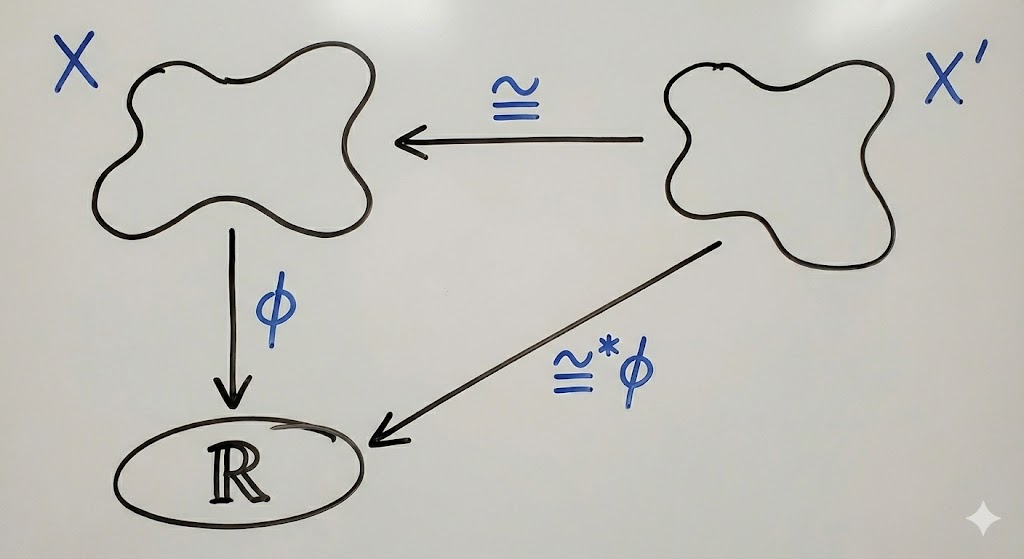
By contrast, for \(T=v\) a vector field on \(X\), one naturally demands \(v’\in\mathfrak{X}(X’)\) to obey \(v'(\phi’)(x’)=v(\phi)(x)\). Again, because \(\cong\) is assumed to be a diffeomorphism, \(v\) can be transported from \(X\to X’\) via either a pushforward or a pullback, but unlike for scalar fields, here it turns out (why?) to be more natural to use a pushforward \(\cong:X\to X’\) so that \(v’=\cong_*v\), \(\phi=\cong^*\phi’\), and \(x’=\cong(x)\).
If \(x^{\mu}\) is some chart on \(X\) with respect to which \(v=v^{\mu}\partial_{\mu}\), and \(x’^{\mu}\) is some chart on \(X’\) (note that generically \(x^{\mu}\neq\cong^*x’^{\mu}\)), then the components of the pushforward are given by:
\[(\cong_*v)^{\mu}(x’)=\frac{\partial x’^{\mu}}{\partial x^{\nu}}v^{\nu}(x)\]
Problem: Let \(X\) be a smooth manifold, let \(\phi\in C^{\infty}(X)\) be a scalar field on \(X\), and let \(v\in\mathfrak{X}(X)\) be a vector field flowing on \(X\). Explain how the scalar field \(\mathcal L_v(\phi)\in C^{\infty}(X)\) is defined (this is called the Lie derivative of \(\phi\) “along” \(v\)), and how it is calculated.
Solution: Recall that for a scalar field \(\phi(\mathbf x)\) on \(\mathbf x\in\mathbf R^n\), the directional derivative of \(\phi\) along a velocity vector \(\mathbf v\in\mathbf R^n\) is defined by the limit:
\[\lim_{t\to 0}\frac{\phi(\mathbf x+t\mathbf v)-\phi(\mathbf x)}{t}=\left(\frac{d\phi(\mathbf x+t\mathbf v)}{dt}\right)_{t=0}=\mathbf v\cdot\frac{\partial\phi}{\partial\mathbf x}\]
By analogy, one defines:
\[\mathcal L_v\phi(x):=\lim_{t\to 0}\frac{v_t^*\phi(x)-\phi(x)}{t}=\left(\frac{d\phi(v_t(x))}{dt}\right)_{t=0}=v(\phi)(x)\]
Thus, \(\mathcal L_v\phi=v(\phi)\), or more abstractly (remembering this is the Lie derivative \(\mathcal L_v:C^{\infty}(X)\to C^{\infty}(X)\) on scalar fields) \(\mathcal L_v=v\).
Problem: Repeat the above for the action of the Lie derivative \(\mathcal L_v\) on another vector field \(v’\in\mathfrak{X}(X)\) to produce the vector field \(\mathcal L_v(v’)\in\mathfrak{X}(X)\).
Solution: The basic idea is that tangent vectors living in distinct tangent spaces cannot be subtracted. So one has to pushforward the future tangent vector “back in time”:
\[\mathcal L_vv’:=\lim_{t\to 0}\frac{(v^{-1}_t)_*v’-v’}{t}\]
One way to proceed is to define an auxiliary scalar field \(f(t,t’):=v'(\phi\circ v_{-t})(v_{t’}(x))\) in which case one can use the chain rule to compute \(\mathcal L_vv'(\phi)(x)=\left(\frac{df(t,t)}{dt}\right)_{t=0}=\left(\frac{\partial f(t,0)}{\partial t}\right)_{t=0}+\left(\frac{\partial f(0,t’)}{\partial t’}\right)_{t’=0}\). However, here it will be fun to directly Maclaurin expand the numerator of the limit. Recall from earlier the fundamental property of infinitesimal flows \(\text{test scalar field}(v_t(x))\approx\text{test scalar field}(x)+tv(\text{test scalar field})(x)\). First, apply it to \(\text{test scalar field}=v'(\phi\circ v_{-t})\):
\[v'(\phi\circ v_{-t})(v_t(x))\approx v'(\phi\circ v_{-t})(x)+tv(v'(\phi\circ v_{-t}))(x)\]
Then apply it again for \(\text{test scalar field}=\phi\) and replace \(t\mapsto -t\):
\[\phi\circ v_{-t}\approx \phi-tv(\phi)\]
Distributing everything up to \(O(t)\), using linearity of vector fields, the limit reduces to \(\mathcal L_vv’=[v,v’]\). More abstractly, the Lie derivative is just the Lie bracket (hence the name!) on \(\mathfrak{X}(X)\), i.e. \(\mathcal L_v=[v,\space]\). Indeed, one can check that it is a Lie algebra representation because of the homomorphism property \(\mathcal L_{[v,v’]}=[\mathcal L_v,\mathcal L_{v’}]\) thanks to the Jacobi identity.
Problem: Define a covector at some point \(x\in X\) on a \(C^1\)-manifold \(X\). Hence, define a \(1\)-form on \(X\). Clearly emphasize the difference between a covector and a \(1\)-form.
Solution: At \(x\in X\), one of course has the tangent space \(T_x(X)\). Since \(T_x(X)\) is a vector space, it has an associated dual vector space \(T^*_x(X)\) which in this context is called the cotangent space at \(x\in X\) (cf. \(\tan\) vs. \(\cot\)). As the linear functionals \(v_x\in T_x(X)\) are called tangent vectors at \(x\in X\), so it makes sense that the linear functionals \(A_x\in T^*_x(X)\) are called cotangent vectors at \(x\in X\), or covectors for short.
Just as a (tangent) vector field \(v\) assigns a tangent vector \(v_x\in T_x(X)\) to each point \(x\in X\) across the manifold \(X\), a (cotangent) vector field \(\omega\) assigns a cotangent vector \(A_x\in T_x^*(X)\) to each point \(x\in X\). This “covector field” is called a differential \(1\)-form, or \(1\)-form for short.
Problem: Show how, by applying the exterior derivative \(d\) to any scalar field \(\phi\in C^{\infty}(X)\cong\Omega^0(X)\) (also called a differential \(0\)-form), the resulting object \(d\phi\in\Omega^1(X)\) is a \(1\)-form.
Solution: This is because \(d\phi\) is defined by its action on an arbitrary vector field \(v\) as:
\[d\phi(v):=v(\phi)=\mathcal L_v(\phi)\]
Problem: Explain why, when the manifold \(X\) is covered by a coordinate chart \((x^0,…,x^{n-1})\), any exact differential \(1\)-form is given by the familiar chain rule:
\[d\phi=\frac{\partial\phi}{\partial x^{\mu}}dx^{\mu}\]
Solution: The first thing is to unpack the meaning of the differentials \(dx^{\mu}\). This amounts to substituting \(\phi=x^{\mu}\) for the exterior derivative of a \(0\)-form, so for an arbitrary vector field \(v\), one has:
\[dx^{\mu}(v):=v(x^{\mu})\]
In particular, if \(v=\partial_{\nu}\) for some \(\nu\), then \(\partial x^{\mu}/\partial x^{\nu}=\delta^{\mu}_{\nu}\), so \(dx^{\mu}\) is the dual coordinate basis for \(\Omega^1(X)\) with respect to the coordinate basis \(\partial_{\mu}\) of \(\mathfrak{X}(X)\). The components of \(d\phi\) in the \(dx^{\mu}\) basis are thus as claimed:
\[d\phi=d\phi(\partial_{\mu})dx^{\mu}=\partial_{\mu}\phi dx^{\mu}\]
Problem: Let \(X\) be a \(C^1\)-manifold and let \(x^{\mu}\) and \(x’^{\mu}\) be two coordinate charts for \(X\). Compare how the vector field basis, the one-form basis, and the components of vectors and one-forms in their respective bases transform between these \(2\) coordinate charts.
Solution: Let \(v=v^{\mu}\partial_{\mu}=v’^{\mu}\partial’_{\mu}\) be a vector field and \(A=A_{\mu}dx^{\mu}=A’_{\mu}dx’^{\mu}\) be a \(1\)-form. In what follows, the key is to always remember that the underlying objects \(v, A\) are chart-invariant, so if the basis transforms under one particular Jacobian, then the components must transform under the inverse Jacobian.
One can start with the vector field basis \(\partial’_{\mu}=\partial’_{\mu}x^{\nu}\partial_{\nu}\) which is just the indisputable chain rule. With that as an anchoring point, one immediately concludes \(v’^{\mu}=\partial_{\nu}x’^{\mu}v^{\nu}\). Then, by enforcing that \(dx’^{\mu}(\partial’_{\nu})=\delta^{\mu}_{\nu}\) remains biorthogonal, this leads to the intuitive chain rule requirement \(dx’^{\mu}=\partial_{\nu}x’^{\mu}dx^{\nu}\), and hence \(A’_{\mu}=\partial’_{\mu}x^{\nu}A_{\nu}\).
Problem: Let \(X\) and \(X’\) be smooth, diffeomorphic manifolds. Earlier it was seen that scalar fields are naturally transported via pullback whereas vector fields are naturally transported via pushforward. What about for \(1\)-forms? Hence, define the Lie derivative \(\mathcal L_vA\) of a \(1\)-form \(A\) with respect to a vector field \(v\).
Solution: Just like scalar fields, \(1\)-forms naturally pullback (can remember this because they both map to \(\mathbf R\)). Specifically, if \(A\in\Omega^1(X)\) currently lives on \(X\), and one has a diffeomorphism \(\cong:X’\to X\), then:
\[\cong^*A(v):=A(\cong_*v)\]
Or in components (using the earlier result for vector field pushforward components \((\cong_*v)^{\mu}(x’)=\frac{\partial x’^{\mu}}{\partial x^{\nu}}v^{\nu}(x)\)):
\[(\cong^*A)_{\mu}=\frac{\partial x’^{\nu}}{\partial x^{\mu}}A_{\nu}\]
The Lie derivative is then given by:
\[\mathcal L_{v}A:=\lim_{t\to 0}\frac{v_t^*A-A}{t}\]
It turns out (how?) one can show that \(\mathcal L_v A=(\mathcal L_v A)_{\mu}dx^{\mu}\) where the components are:
\[(\mathcal L_v A)_{\mu}=v^{\nu}\partial_{\nu}A_{\mu}+A_{\nu}\partial_{\mu}v^{\nu}\]
Problem: Let \(X\) be a smooth \(n\)-manifold, and let \(x\in X\). Define a tensor \(T_x\) of type \((k^*,k)\) (i.e. rank \(k^*+k\)) at \(x\). Define the components of the tensor \(T_x\) with respect to a suitable ordered basis. Give an example of a tensor field defined over any manifold \(X\).
Solution: Just as vector fields are smooth assignments of tangent vectors across \(X\), just as \(1\)-forms are smooth assignments of covectors across \(X\), tensor fields are smooth assignments of tensors across \(X\). In particular, it only makes sense to speak of a tensor \(T_x\) at a specific point \(x\in X\), and to view the object \(T\) itself as a tensor field. With that in mind, a tensor at \(x\in X\) of type \((k^*,k)\in\mathbf N^2\) is defined (at least in differential geometry) to be any multilinear map \(T_x:T^*_x(X)^{k^*}\times T_x(X)^k\to\mathbf R\) that eats in \(k^*\) covectors in the cotangent space \(T^*_x(X)\) and \(k\) tangent vectors in the tangent space \(T_x(X)\) and spits out a scalar. The corresponding tensor field can be viewed as a map \(T:\Omega^1(X)^{k^*}\times\mathfrak{X}(X)^k\to C^{\infty}(X)\). Given an ordered (possibly non-coordinate) basis \(\partial_{\mu}\) for \(\mathfrak{X}(X)\) with corresponding dual ordered (again! possibly non-coordinate) basis \(dx^{\mu}\) for \(\Omega^1(X)\), the \(n^{k^*+k}\) components of \(T\) are defined by:
\[T^{\mu_1,…,\mu_{k^*}}_{\nu_1,…,\nu_{k}}:=T(dx^{\mu_1},…,dx^{\mu_{k^*}},\partial_{\nu_1},…,\partial_{\nu_{k}})\]
Thus, covectors are type \((0,1)\) tensors while tangent vectors are type \((1,0)\) tensors. Any manifold \(X\) is equipped with a type \((1,1)\) tensor field \(\delta:\Omega^1(X)\times\mathfrak{X}(X)\to C^{\infty}(X)\) defined by:
\[\delta(A,v):=A(v)\Leftrightarrow\delta(dx^{\mu},\partial_{\nu})=\delta^{\mu}_{\nu}\]
Problem: (tensor component transformation)
Solution:
Problem: Let \(T,T’\) be respectively type \((k^*,k)\) and \((k’^*,k’)\) tensor fields defined over the same smooth \(n\)-manifold \(X\). Define the \((k^*+k’^*,k+k’)\) tensor field given by their tensor product \(T\otimes T’:\Omega^1(X)^{k^*+k’^*}\times\mathfrak{X}(X)^{k+k’}\to C^{\infty}(X)\).
Solution: It’s pretty much the obvious thing one can write down that sums the tensor ranks:
\[T\otimes T'(A_1,…,A_{k^*},A’_1,…,A’_{k’^*},v_1,…,v_k,v’_1,…,v’_{k’})\]
\[:=T(A_1,…,A_{k^*},v_1,…,v_k)T'(A’_1,…,A’_{k’^*},v’_1,…,v’_{k’})\]
Or, with respect to an ordered (possibly non-coordinate!) basis \(\{\partial_{\mu}\}\) of \(\mathfrak{X}(X)\):
\[(T\otimes T’)^{\mu_1,…,\mu_{k^*},\mu’_1,…,\mu’_{k’^*}}_{\nu_1,…,\nu_k,\nu’_1,…,\nu’_{k’}}=T^{\mu_1,…,\mu_{k^*}}_{\nu_1,…,\nu_k}T’^{\mu’_1,…,\mu’_{k’^*}}_{\nu’_1,…,\nu’_{k’}}\]
Problem: Show how to compute the pushforward \(\cong_*T\) of a tensor field \(T\), and hence show how to take the Lie derivative \(\mathcal L_{\partial}T\) of a tensor field \(T\) along a vector field \(\partial\).
Solution:
Problem: Define a differential \(k\)-form.
Solution: Differential \(k\)-forms are simply antisymmetric type \((0,k)\) tensor fields. At each point \(x\in X\), one can think of them as measuring devices that eat in \(k\) tangent vectors in \(T_x(X)\) and spit out a number. More globally, \(\omega\in\Omega^k(X)\) is said to be a differential \(k\)-form iff \(\omega:\mathfrak{X}(X)\to C^{\infty}(X)\) takes in \(k\) vector fields and spits out a scalar field.
Problem: Given a differential \(k\)-form \(\omega\in\Omega^k(X)\) and a differential \(k’\)-form \(\omega’\in\Omega^{k’}(X)\), define the differential \(k+k’\)-form given by their wedge product \(\omega\wedge\omega’\in\Omega^{k+k’}(X)\).
Solution:
Problem: Define the exterior derivative \(d:\Omega^k(X)\to\Omega^{k+1}(X)\) of a differential \(k\)-form, showing how it generalizes the earlier definition given for \(k=0\)-forms.
Solution: Recall that the wedge product \(\wedge\) of a differential \(k’\)-form and a differential \(k\)-form is a differential \(k’+k\)-form. In particular, the exterior derivative can loosely be viewed as a special case of the wedge product with \(k’=1\) and \(d=\partial_{\mu}dx^{\mu}\wedge\); for instance \(d\phi=\partial_{\mu}dx^{\mu}\), and for a \(1\)-form \(A=A_{\mu}dx^{\mu}\) the exterior derivative \(F:=dA\) is given by:
\[F=\partial_{\mu}dx^{\mu}\wedge A_{\nu}dx^{\nu}=\partial_{\mu}A_{\nu}dx^{\mu}\wedge dx^{\nu}=\frac{1}{2}F_{\mu\nu}dx^{\mu}\wedge dx^{\nu}\]
with \(F_{\mu\nu}:=\partial_{\mu}A_{\nu}-\partial_{\nu}A_{\mu}\).
Problem: Prove the following properties of the wedge product \(\wedge\) and its interaction with the exterior derivative \(d\), the pushback, pushforward, tensor product, interior product…?
- (Antisymmetry of odd-degree forms) \[\omega\wedge\omega’=(-1)^{kk’}\omega’\wedge\omega\]
- (Graded product rule with respect to \(d\)) \[d(\omega\wedge\omega’)=(d\omega)\wedge\omega’+(-1)^k\omega\wedge d\omega’\]
Problem: Prove Cartan’s magic formula:
\[\mathcal L_{\partial}=\{d,\iota_{\partial}\}\]