
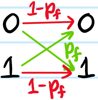
Problem: Draw a schematic of a binary symmetric channel (BSC) with bit flip probability \(p_f\).
Solution: Classically, one has:
On the other hand, taking a more quantum perspective, in the computational basis \((|0\rangle,|1\rangle)\) one might define a binary symmetric channel as a kind of quantum logic gate:
\[\text{BSC}_{p_f}=\begin{pmatrix}\sqrt{1-p_f}&\sqrt{p_f}\\\sqrt{p_f}&\sqrt{1-p_f}\end{pmatrix}\]
The word “symmetric” in the name emphasizes that the bit flip probability from \(0\to 1\) is identical to the bit flip probability \(1\to 0\).
Problem: Consider the radio communication link between Galileo and Earth, and suppose that the noisy communication channel between them may be modelled as a BSC with bit flip probability \(p_f=0.01\). In a sequence of \(N=10^5\) bit transmissions, what is the probability that the error rate is less than \(1\%\)?
Solution: This means that one requires \(N'<0.01N=10^3\) bit flips. Each such \(N’\) has binomial probability \({{N}\choose{N’}}p_f^{N’}(1-p_f)^{N’}\) so the total probability is given by the cumulative distribution function:
\[\sum_{N’=0}^{N’=999}{{N}\choose{N’}}p_f^{N’}(1-p_f)^{N’}\]
Problem: What are the \(2\) solutions for addressing noise in communication channels? Which one is preferable?
Solution:
- The physical solution: build more reliable hardware, cooling circuits, etc. (basically all the stuff one learns in a typical experimental physics class).
- The system solution: accept the noisy communication channel as is, and add communication systems to it so as to detect and correct errors. This is the goal of coding theory.
The system solution is preferable because it only comes at an increased computational cost whereas the former comes at an increased financial cost. But more importantly, the improvements arising from the system solution can be very dramatic, unlike the incremental improvements of the physical solution.
Problem: What is the distinction between information theory and coding theory?
Solution: The difference between information theory and coding theory is analogous to the distinction between theoretical physics and experimental physics; the former is concerned with the theoretical limitations of the aforementioned communication systems (e.g. “what is the best error-correcting performance possible over the space of all possible error-correcting algorithms?”) whereas the latter is interested in specifically designing practical such algorithms (also called codes) for error correction.
Problem: Draw a schematic that depicts the high-level structure of an error-correcting code.
Solution: Coding = Encoding + Decoding:
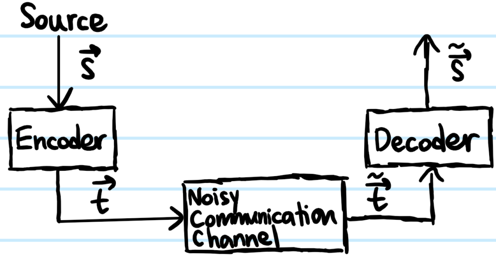
Here \(\mathbf s\) is the source message vector which is encoded as a transmitted message vector \(\mathbf t=\mathbf s+\textbf{redundancy}\). After transmission across the noisy communication channel, the transmitted message vector has been distorted into \(\tilde{\mathbf t}=\mathbf t+\textbf{noise}\). This is then decoded and received as a message vector \(\tilde{\mathbf s}\) with the hope that \(\tilde{\mathbf s}=\mathbf s\) with probability close to \(1\).
Problem: Consider a first naive attempt at designing an error-correcting code for a BSC, known as a repetition code. Explain how that works with an example.
Solution: A choice of error-correcting code basically amounts to a choice of encoder + decoder, since again coding = encoding + decoding. For the repetition code, the encoder is literally a repetition of each bit a predefined number of times, say \(3\) in the example below. The corresponding optimal decoder turns out to be the obvious “majority-vote” among the triplets (assuming \(p_f<1/2\); if it were the case that \(p_f>1/2\) then instead a “minority-vote” decoder would be better!)
(aside: “optimal” means the decoder should map each \(\tilde{\mathbf t}\) to \(\tilde{\mathbf s}=\text{argmax}_{\mathbf s}p(\mathbf s|\tilde{\mathbf t})\) and in particular as part of computing this conditional probability, another implicit assumption is that both \(p(0)=p(1)=1/2\) have equal prior probabilities)
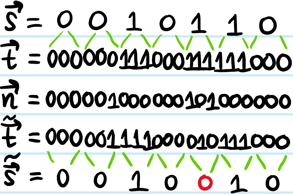
Here \(\mathbf n\) is a spare noise vector each of whose bits are sampled from a \(p_f\)-Bernoulli distribution, where \(0\) means no bit flip and \(1\) means yes bit flip, and \(\tilde{\mathbf t}\equiv\mathbf t+\mathbf n\pmod{2}\), or using the xor notation, \(\tilde{\mathbf t}=\mathbf t\oplus\mathbf n\)
Problem: Show that, compared to no repetition for which the bit flip probability across the BSC is \(p_f<1/2\), the \(3\)-fold repetition code has an effective bit flip probability \(p^{\text{eff}}_f<p_f\) which is reduced compared to the original bit flip probability \(p_f\).
Solution: In order to get a bit flip, either \(2\) or all \(3\) bits in the \(3\)-fold repetition encoded vector \(\mathbf t\) have to be flipped. Thus, the effective bit flip probability \(p^{\text{eff}}_f\) is a cubic function of \(p_f\):
\[p^{\text{eff}}_f=3p_f^2(1-p_f)+p_f^3=3p_f^2-2p_f^3\]
In order to have \(p^{\text{eff}}_f<p_f\), this requires:
\[3p_f-2p_f^2<1\Rightarrow 2(p_f-1/2)(p_f-1)>0\]
which is satisfied for \(p_f<1/2\).
Problem: Instead of \(N=3\) repetitions, generalize the above expression for the effective bit flip probability \(p^{\text{eff}}_f\) to an arbitrary odd number \(N\) of repetitions.
Solution: The effective bit flip probability \(p^{\text{eff}}_f\) is now a degree-\(N\) polynomial in \(p_f\):
\[p^{\text{eff}}_f=\sum_{n=(N+1)/2}^N{N\choose n}p_f^n(1-p_f)^{N-n}\]
which for \(p_f\ll 0.5\) is dominated by the first term \(n=(N+1)/2\).
Problem: Describe how the \((7,4)\) Hamming error correction code works, and explain why it’s an example of a linear block code.
Solution: The idea is that if the source vector \(\mathbf s\) has length \(L_{\mathbf s}\) and the encoded transmitted vector \(\mathbf t\) has some larger length \(L_{\mathbf t}>L_{\mathbf s}\), then one has the “rate” \(L_{\mathbf s}/L_{\mathbf t}=4/7\). Specifically, for every \(4\) source bits \(\mathbf s=s_1s_2s_3s_4\), the transmitted vector will contain \(7\) bits \(\mathbf t=t_1t_2t_3t_4t_5t_6t_7\) such that \(t_{1,2,3,4}:=s_{1,2,3,4}\) and \(t_{5,6,7}\) are uniquely specified by the requirements that \(t_1+t_2+t_3+t_5\equiv t_2+t_3+t_4+t_6\equiv t_1+t_3+t_4+t_7\equiv 0\pmod 2\); in other words, \(t_{5,6,7}\) are said to be parity-check bits in the sense that they check the parity of a certain subset of the source bits \(s_{1,2,3,4}\). This encoding can be depicted visually as such:
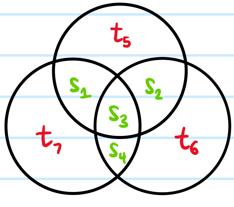
where the parity of each of the \(3\) circles has to be even. For example, if \(\mathbf s=1011\), then the Hamming encoding of this would be \(\mathbf t=1011001\).
As for the \((7,4)\) Hamming decoder, for generic \(p_f<1/2\) it can be a bit tricky but if one assumes \(p_f\ll 1/2\), then it is pretty safe to assume that there will be at most \(1\) bit flip during transmission across the noisy binary symmetric communication channel \(\mathbf t\mapsto\tilde{\mathbf t}\). In that case, one can take a given \(\tilde{\mathbf t}\) and compute its syndrome vector \(\mathbf z\); i.e. in each of the \(3\) circles, has the parity remained even \((0)\) or has it become odd \((1)\)? For instance, getting a syndrome \(\mathbf z=000\) means that most likely no bits were flipped and thus there are no errors! Or, if \(\mathbf z=011\), then under the premise that there was only a single bit flip, it must have been \(s_4\), etc. In general, \(\tilde{\mathbf t}\) can have \(8\) possible syndromes \(\mathbf z\), and each such syndrome \(\mathbf z\) maps uniquely onto the \(7\) possible single bit flips together with the possibility of zero bit flips.
The Hamming code is a block code because the parity-check bits look at whole blocks (or subsets) of the source bitstring \(\mathbf s\), rather than one bit of \(\mathbf s\) at a time (as was essentially done in repetition coding). The Hamming code is also said to be a linear code (mod \(2\)) because the encoding operation is linear in the sense that (assuming \(\mathbf s,\mathbf t\) are both column vectors):
\[\mathbf t=G^T\mathbf s\]
where the \(7\times 4\) generator matrix is given by:
\[G^T=\begin{pmatrix}1&0&0&0\\0&1&0&0\\0&0&1&0\\0&0&0&1\\1&1&1&0\\0&1&1&1\\1&0&1&1\end{pmatrix}\]
Or transposing both sides, \(\mathbf t^T=\mathbf s^TG\), and in some coding theory texts one often takes \(\mathbf s,\mathbf t\) to be row vectors by default in which case this would just be written \(\mathbf t=\mathbf sG\). Of course, the columns of \(G^T\) represent the encodings \(\mathbf t\) of the “basis” bitstrings \(\mathbf s=1000,0100,0010,0001\).
Problem: The \((7,4)\) Hamming decoder \(\tilde{\mathbf t}\to\mathbf z\to\tilde{\mathbf s}\) uses a syndrome vector \(\mathbf z\) as an intermediate in the decoding process. Show that the map from \(\tilde{\mathbf t}\to\mathbf z\) is linear in the sense that:
\[\mathbf z=H\tilde{\mathbf t}\]
where the parity-check matrix \(H:=(P,1_3)\), and \(P=\begin{pmatrix}1&1&1&0\\0&1&1&1\\1&0&1&1\end{pmatrix}\) also appears in the generator matrix via:
\[G^T=\begin{pmatrix}1_4\\P\end{pmatrix}\]
Show that \(HG^T=0\) and hence if there were no errors such that \(\tilde{\mathbf t}=\mathbf t\), then the corresponding syndrome vector \(\mathbf z=\mathbf 0\Leftrightarrow\mathbf t\in\text{ker}H\). Hence, explain why a maximum-likelihood decoder is equivalent to finding the most probable noise vector \(\mathbf{n}\) for which \(\mathbf z=H\mathbf n\).
Solution: Just check it, it’s true. And clearly \(HG^T=2P=0\) because \(2\equiv 0\pmod 2\). It follows then that \(\mathbf t\in\text{ker}H\) because \(\mathbf t=G^T\mathbf s\). Thus, because \(\tilde{\mathbf t}=\mathbf t+\mathbf n\), acting on both sides with \(H\) results in \(\mathbf z=H\mathbf n\).
Problem: As the \((7,4)\) Hamming code is a block code, given a possibly very long source message, the only way to implement the code is to chop up the message into blocks of length \(L_{\mathbf s}=4\); naturally, one can ask, for any given block in this “assembly line”, what’s the probability \(p(\tilde{\mathbf s}\neq\mathbf s)\) of it being decoded incorrectly? By contrast, a different question one can ask is what is the effective bit flip probability \(p_f^{\text{eff}}\) within one of these blocks? (give both to leading order in \(p_f\))
Solution: First, notice that without the Hamming code, any odd number of bit flips as well as certain combinations of an even number of bit flips would lead very easily to a decoding error \(\tilde{\mathbf s}\neq\mathbf s\); as \(p_f\ll 1/2\), the dominant process is having a single bit flip, so in this case \(p(\tilde{\mathbf s}\neq\mathbf s)={4\choose{1}}p_f(1-p_f)^3+…=4p_f+O(p_f^2)\).
By contrast, with the \((7,4)\) Hamming code, the block error probability is no longer linear in \(p_f\), but quadratic. This is simply because the \((7,4)\) Hamming code is designed to correct all \(1\)-bit flip errors, thereby eradicating the dominant process above. Unfortunately, any \(2\) bit flips (implicitly on distinct bits) in the \(7\)-bit encoding \(\mathbf t\) will not be corrected, leading to block error \(\tilde{\mathbf s}\neq\mathbf s\) (identical remarks apply to \(3,4,5,6,7\) bit flips); after all, no matter what syndrome vector \(\mathbf z\) one finds in \(\tilde{\mathbf t}\), the Hamming decoder tells one to unflip at most \(1\) bit because it operates under the assumption that there was only \(1\) bit flip, so it is literally impossible to fully correct a \(\tilde{\mathbf t}\) containing more than \(1\) bit flip. Thus:
\[p(\tilde{\mathbf s}\neq\mathbf s)=\sum_{n=2}^7{7\choose{n}}p_f^n(1-p_f)^{7-n}=21p_f^2+O(p_f^3)\]
By contrast, the effective bit flip probability is in general:
\[p_f^{\text{eff}}=\frac{1}{L_{\mathbf s}}\sum_{i=1}^{L_{\mathbf s}}p(\tilde s_i\neq s_i)\]
But here all \(L_{\mathbf s}=4\) source bits are indistinguishable (indeed all \(L_{\mathbf t}=7\) transmitted bits are indistinguishable), so one can focus arbitrarily on e.g. \(i=1\) and ask what is \(p_f^{\text{eff}}=p(\tilde s_1\neq s_1)\). There are then \(2\) distinct ways to obtain the same answer (to leading order); the first is to explicitly enumerate all the possible \(2\) bit flip errors in \(\tilde{\mathbf t}\) such that the final decoded source vector \(\tilde{\mathbf s}\) will have an error in bit \(\tilde s_1\neq s_1\); clearly there are \(6\) such combinations that look like \(s_1\) being flipped in addition to one of the other \(6\) bits; then, another \(3^{\text{rd}}\) bit will always be flipped. Meanwhile, one can check there are also \(3\) other configurations in which \(s_1\) is not initially flipped, but rather the decoder incorrectly flips it when going from \(\tilde{\mathbf t}\to\tilde{\mathbf s}\):

Since each of these are still \(2\) bit flip processes, one thus has:
\[p_f^{\text{eff}}=9p_f^2(1-p_f)^5+…=9p_f^2+O(p_f^3)\]
To leading order, one thus observes that \(p_f^{\text{eff}}=\frac{3}{7}p(\tilde{\mathbf s}\neq\mathbf s)\); the \(3/7\) prefactor has a simple interpretation as saying that whenever there was \(2\) bit flips in \(\tilde{\mathbf t}\), it would inevitably imply \(3\) bit flips in the decoded \(\tilde{\mathbf s}\) (prior to truncating away the \(3\) parity-check bits) so \(3\) out of the \(7\) bits in \(\tilde{\mathbf s}\) are in error, and all \(7\) bits are indistinguishable. This thus has a very Bayesian interpretation where \(p(\tilde{\mathbf s}\neq\mathbf s)\) is the prior and \(3/7\) is the conditional probability of a bit like \(s_1\) being flipped if it’s known that the whole \(7\)-bit block has suffered a \(3\)-bit error.
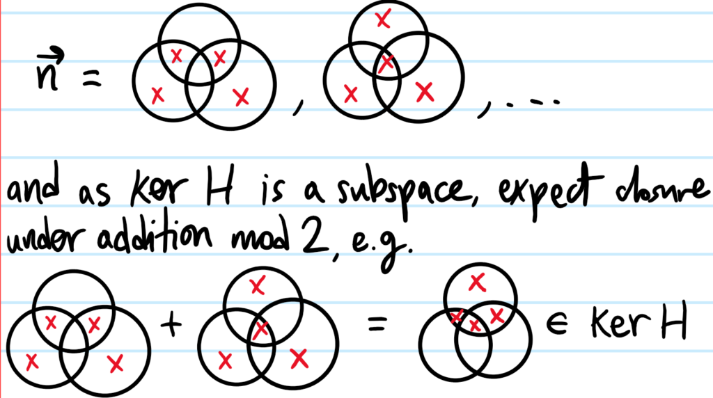
Problem: How many distinct elements are there in \(\ker H\)? What is the interpretation of such an element?
Solution: There are \(15\) elements in \(\ker H\), and each such \(\mathbf n\in\ker H\) has the property that the corresponding syndrome \(\mathbf z=\mathbf 0\) if \(\textbf n\) were interpreted as a certain symmetric pattern of bit flips/noise. For example:
Problem: The \((7,4)\) Hamming code is not the only one; what other possible \((L_{\mathbf t},L_{\mathbf s})\) Hamming codes are possible?
Solution: Any for which \(L_{\mathbf t}-L_{\mathbf s}=\log_2(L_{\mathbf t}+1)\), the RHS being the number of parity-check bits which grows merely logarithmically with the total transmission size \(L_{\mathbf t}\)!
Problem: What are the \(2\) main interpretations of probability?
Solution: There is the frequentist and Bayesian interpretations of probability; the former interprets probabilities as long-run event frequencies while the latter inteprets probabilities as degrees of belief (this is possible provided the concept of “degree of belief” satisfies certain reasonable Cox axioms). In general, probability theory is simply an extension of logic to account for uncertainty.
Problem: Whenever dealing with multiple random variables \(X,Y,…\), what is the fundamental object to look at? What can be derived from this fundamental object? (cf. the partition function in statistical mechanics as serving the same sort of “all-encompassing” role).
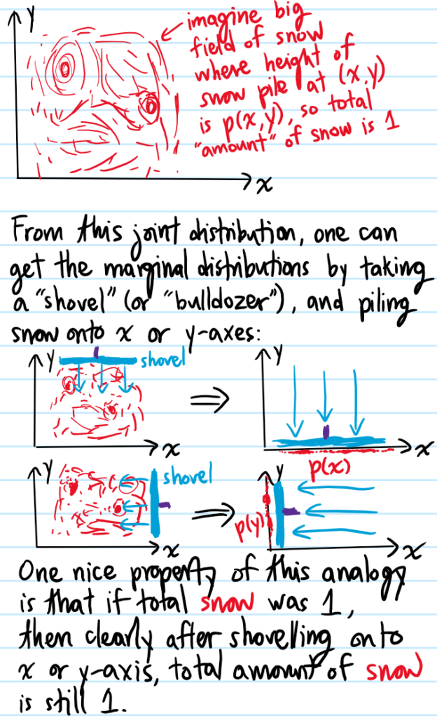
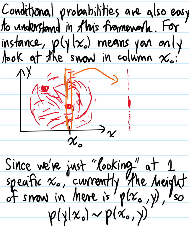
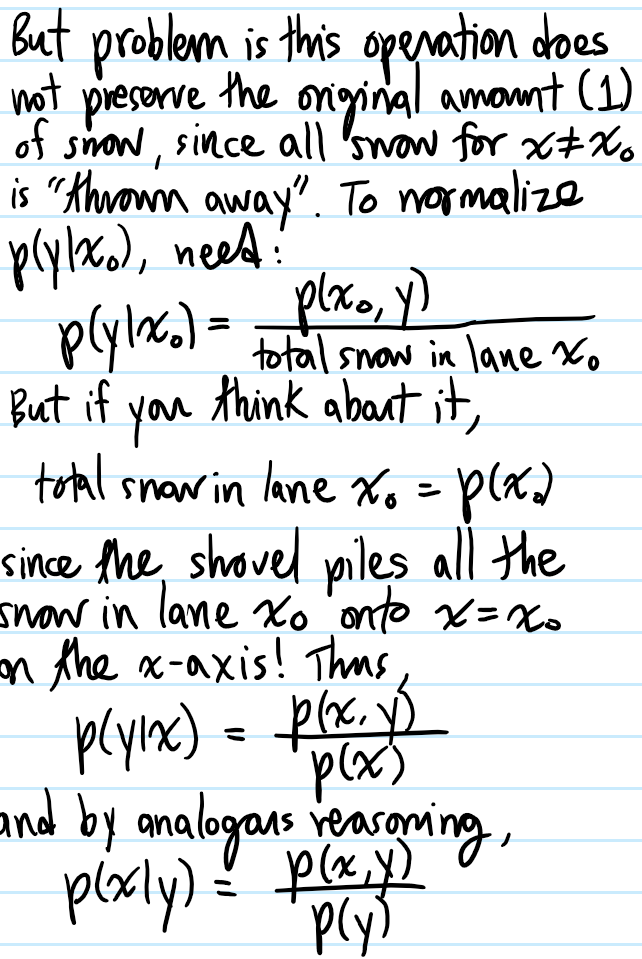
Solution: The fundamental object which one should prioritize figuring out is the joint probability distribution function \(p_{(X,Y,…)}(x,y,…)\) of all the random variables \((X,Y,…)\). Consider a simple visualization of this concept for just \(2\) real-valued random variables \(X, Y\) and the marginal as well as conditional probability distributions one can obtain from their joint probability distribution \(p_{(X,Y)}(x,y)\equiv p(x,y)\):
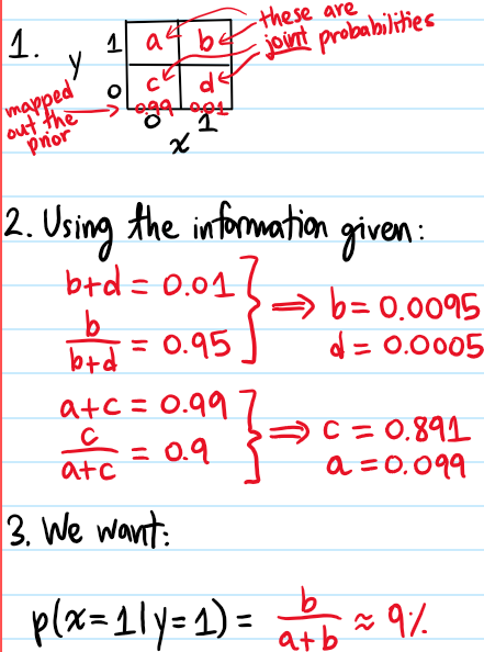
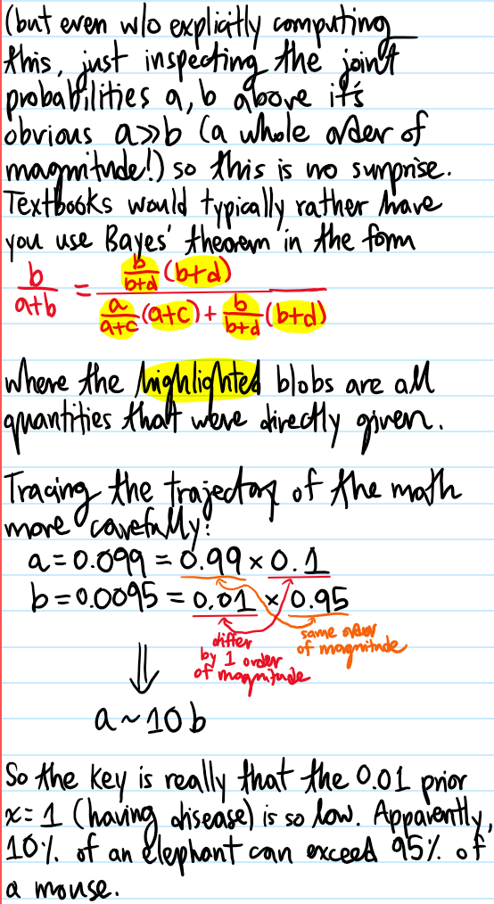
Problem: A certain disease is present among \(1\%\) of the world’s population, and a medical test for the disease has a \(95\%\) true positive rate and a \(90\%\) true negative rate. If Joe tests positive for the disease, what are his odds of actually having it?
Solution: For these sorts of problems, there is essentially a \(3\)-step recipe to solving them:
- Map out the complete marginal distribution of the prior.
- For each value of the prior, “unshovel” your way back to the joint distribution w.r.t. all values of the new data.
- Hence, compute whatever you need to.
In this case, the prior \(X\) may be modelled as a Bernoulli random variable taking on the value \(x=0\) if a person doesn’t have the disease and \(x=1\) if they do. Following the steps:
Problem: Suppose that on a certain online store, products can be rated either positively or negatively. There are \(3\) different sellers of the same product. Seller \(A\) has \(10\) reviews with \(100\%\) positive ratings, seller \(B\) has \(50\) reviews with \(96\%\) positive ratings, and seller \(C\) has \(200\) reviews with \(93\%\) positive ratings. Which seller should one buy from?
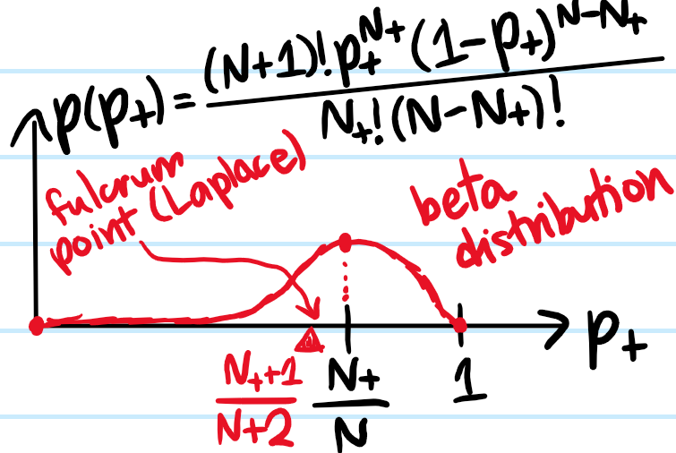
Solution: This is another Bayesian inference problem (draw a picture with \(p_+\) on the horizontal axis and \(N_+\) on the vertical axis!). The model is that the seller has some underlying fixed, but unknown probability \(p_+\) of delivering a positive experience and \(1-p_+\) of delivering a negative experience to a user. A priori, if one had no knowledge about the review information of other customers, then the prior \(p_+\) can be modelled by a uniform distribution \(p(p_+)=1\) for \(p_+\in[0,1]\). But then, equipped with the review info of \(N_+\) positive reviews out of \(N\), Bayesian updating says that this uniform prior should be updated to a beta distributed posterior:
\[p(p_+|N_+,N)=\frac{p(p_+)p(N_+,N|p_+)}{\int_0^1dp_+p(p_+)p(N_+,N|p_+)}=\frac{{N\choose{N_+}}p_+^{N_+}(1-p_+)^{N-N_+}}{\int_0^1 dp_+{N\choose{N_+}}p_+^{N_+}(1-p_+)^{N-N_+}}=\frac{(N+1)!p_+^{N_+}(1-p_+)^{N-N_+}}{N_+!(N-N_+)!}\]
where the beta function \(\textrm{B}(z,w):=\int_0^1 dx x^{z-1}(1-x)^{w-1}=\frac{\Gamma(z)\Gamma(w)}{\Gamma(z+w)}\) normalization has been (optionally) used.
A reasonable goal would be to maximize one’s own probability of a positive experience. This means taking the posterior \(p(p_+|N_+,N)\) computed above and recycling that as one’s prior \(p(p_+|N_+,N)\mapsto p(p_+)\). Then, the probability \(p(+)\) of a positive experience coincides with the expected value of \(p_+\):
\[p(+)=\int_0^1 dp_+p(p_+)p_+=\frac{\textrm{B}(N_++2,N-N_++1)}{\textrm{B}(N_++1,N-N_++1)}=\frac{N_++1}{N+2}\]
this result is called Laplace’s rule of succession, and may be remembered by taking the original \(N\) reviews, and appending \(2\) new fictitious reviews in which one is positive and one is negative. For instance, if a product had no reviews so that \(N=N_+=0\), then reasonably enough Laplace’s rule of succession predicts one to have a \(p(+)=1/2\) probability of a positive experience. Applying it to each of the sellers in the question, one finds that seller \(B\) has the highest probability \(p(+)\), so should vendor with them.
Remember that Bayesian inference is always predicated on assumptions, which above meant a uniform equiprobable ignorance \(p(p_+)=1\) at the very beginning about \(p_+\), though it has been suggested by Jeffreys, Haldane, etc. to use a different prior like \(p(p_+)=\frac{1}{\pi\sqrt{p(1-p)}}\) or \(p(p_+)\sim\frac{1}{p(1-p)}\) to model one’s ignorance. Of course, this would modify how Laplace’s rule of succession looks with each of these priors.
Problem: (for fun!) Prove the earlier beta function relation \(\textrm{B}(z,w):=\int_0^1 dx x^{z-1}(1-x)^{w-1}=\frac{\Gamma(z)\Gamma(w)}{\Gamma(z+w)}\). Show that in the special case of positive integers \(z,w\in\mathbf Z^+\), the result may be derived combinatorially.
Solution:


(loosely speaking, this is reminiscent of the identity for the exponential function \(\exp(z)\exp(w)=\exp(z+w)\) except for the \(\Gamma\) function there is an “extra factor” in the form of the beta function \(B(z,w)\)). In the special case where \(z,w\in\mathbf Z^+\), the initial temptation would be to expand \((1-x)^{w-1}\) using the binomial theorem, but it turns out there is a much cuter way to evaluate the integral by telling a story.
Imagine seeing a random distribution of \(N+1\) balls on the unit interval \([0,1]\), of which \(1\) of them is pink while the other \(N\) are black. There are \(2\) ways they could’ve gotten there. On the one hand, it may be that there were initially \(N+1\) black balls, and then one of them was painted pink at random, and then the balls were thrown altogether onto \([0,1]\). Or it may be that the \(N+1\) black balls were first thrown altogether onto \([0,1]\), and subsequently one of them was painted pink at random. Clearly, these \(2\) processes are equivalent definitions of a discrete random variable \(N_+\) defined as the number of black balls to the left of the pink ball on \([0,1]\). This has probability mass function \(p(N_+)\) in the first story given by:
\[p(N_+)=\int_0^1dp_+p(\text{pink thrown at }p_+)p(N_+|\text{pink thrown at }p_+)\]
\[=\int_0^1 dp_+{N\choose{N_+}}p_+^{N_+}(1-p_+)^{N-N_+}\]
On the other hand, according to the second story, \(N_+=0,1,…,N\) each with uniform probability!
\[p(N_+)=\frac{1}{N+1}\]
Hence it is established that:
\[\int_0^1 dp_+p_+^{N_+}(1-p_+)^{N-N_+}=\frac{N_+!(N-N_+)!}{(N+1)!}\]
which is equivalent to the earlier more general result for \(z,w\in\mathbf C\).
Problem: Given a discrete random variable \(X\) with probability mass function \(p(x)\), define the information content \(I(x)\) associated to drawing outcome \(x\) from \(X\). Hence, define the entropy \(S_X\) of \(X\).
Solution: A picture is worth a thousand words:
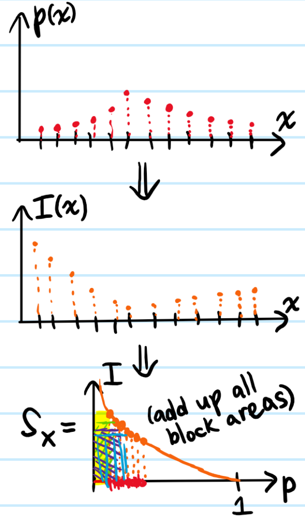
where \(I(x):=-\log p(x)\) is the surprise associated with drawing \(x\) from \(X\), and \(S_X:=\sum_xp(x)I(x)=-\sum_x p(x)\log p(x)=\sum_x I(x)2^{-I(x)}\) is the average surprise of the discrete random variable \(X\). The choice of base in the \(\log\) defines the unit of information (e.g. bits, nats, etc.).
Problem: Show that for \(X\perp Y\) independent discrete random variables, their joint entropy \(S_{(X,Y)}=S_X+S_Y\).
Solution: This is really rooted in Shannon’s fundamental axioms that the joint information content for independent random variables should be additive \(I_{(X,Y)}(x,y)=I_X(x)+I_Y(y)\):
\[S_{(X,Y)}:=-\sum_{(x,y)}p(x,y)\log p(x,y)=-\sum_{(x,y)}p(x)p(y)\log p(x)-\sum_{(x,y)}p(x)p(y)\log p(y)=S_X+S_Y\]
Problem: Give the intuition behind the Kullback-Leibler divergence \(D_{\text{KL}}(\tilde X|X)\) of a random variable \(\tilde X\) with respect to another random variable \(X\) (both defined over the same sample space).
Solution: Any random variable \(X\) inherently contains some non-negative average level of surprise \(S_X\geq 0\) because of the word “random” in “random variable” (indeed, \(S_X=0\) iff \(p(x)=1\) for some outcome \(x\)). That’s one kind of surprise. But in practice, if one is under the illusion that the outcomes \(x\) are being drawn from a random variable \(\tilde X\) when in fact they are actually following a different random variable \(X\neq\tilde X\), then the perceived degree of surprise \(S_{\tilde X|X}=-\sum_xp_X(x)\log p_{\tilde X}(x)\) (called the cross-entropy of \(\tilde X\) with respect to \(X\)) would intuitively be larger than the average surprise \(S_X\) inherent in the intrinsic randomness of \(X\) itself. The KL divergence of \(\tilde X\) with respect to \(X\) thus measures how surprising the data is purely due to the wrong model \(\tilde X\) being used in lieu of the ground truth \(X\):
\[D_{\textrm{KL}}(\tilde X|X):=S_{\tilde X|X}-S_X\]
thus, it should be intuitively clear that \(D_{\textrm{KL}}(\tilde X|X)\geq 0\), a result known as the Gibbs inequality.
Problem: What is the intuition behind Jensen’s inequality.
Solution: Take any “smiling” curve and hang a bunch of masses on the curve. Then Jensen’s inequality says that their center of mass will also lie above the curve.
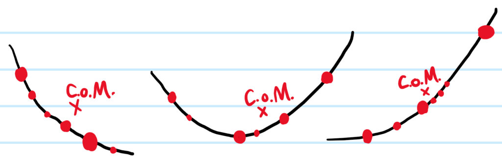
More precisely, for a convex function \(f(x)\) (which means any secant line lies above the function’s graph, or algebraically \(f(\lambda x+(1-\lambda)x’)\leq\lambda f(x)+(1-\lambda)f(x’)\) for \(\lambda\in[0,1]\)), one has:
\[\langle f(x)\rangle\geq f(\langle x\rangle)\]
with equality \(\langle f(x)\rangle=f(\langle x\rangle)\) iff \(x\) is a uniform random variable. More explicitly, for any convex linear combination of the form \(p_1x_1+p_2x_2+…+p_Nx_N\) where each \(p_i\geq 0\) and \(\sum_{i=1}^Np_i=1\), one has:
\[\sum_i p_if(x_i)\geq f\left(\sum_ip_ix_i\right)\]
The inequality is reversed for concave functions \(f(x)\).
Problem: Unstable particles are emitted from a source and decay at a distance \(x\geq 0\), an exponentially distributed real random variable with characteristic length \(x_0\). Decay events can only be observed if they occur in a window extending from \(x=1\) to \(x=20\) (arbitrary units). If \(100\) decays are registered at some locations \(1\leq x_1,x_2,…,x_{100}\leq 20\), estimate the characteristic length \(x_0\).
Solution: The prior distribution of \(x\) is, as stated, an exponential decay:
\[p(x|x_0)=\frac{e^{-x/x_0}}{x_0}[x\geq 0]\]
which is normalized \(\int_{-\infty}^{\infty}dxp(x|x_0)=1\). After learning that \(x\in [1,20]\), the posterior distribution of \(x\) becomes:
\[p(x|x\in [1,20],x_0)=\frac{p(x|x_0)p(x\in[1,20]|x, x_0)}{p(x\in[1,20]|x_0)}\]
but if \(x\) is measured, and happens to lie in \(x\in[1,20]\), then \(p(x\in[1,20]|x, x_0)=1\), otherwise if \(x\notin [1,20]\) then \(p(x\in[1,20]|x, x_0)=0\); all in all one has the compact Iverson bracket expression \(p(x\in[1,20]|x, x_0)=[x\in [1,20]]\). The denominator is the integral of the numerator and indeed is just the usual way that probability density functions are meant to be used:
\[p(x\in[1,20]|x_0)=\int_{-\infty}^{\infty}dxp(x|x_0)p(x\in[1,20]|x,x_0)=\int_1^{20}dx\frac{e^{-x/x_0}}{x_0}=e^{-1/x_0}-e^{-20/x_0}\]
Now, using this updated prior, one has:
\[p(\{x_1,…,x_N\}|x\in[1,20],x_0)=p(x_1|x\in[1,20],x_0)…p(x_N|x\in[1,20],x_0)=\frac{e^{-(x_1+…+x_N)/x_0}}{x_0^N(e^{-1/x_0}-e^{-20/x_0})^N}\]
But one would instead like to Bayesian-infer \(p(x_0|\{x_1,…,x_N\},x\in[1,20])\) so as to find the most probable value of the characteristic length \(x_0\):
\[p(x_0|\{x_1,…,x_N\},x\in[1,20])=\frac{p(x_0|x\in[1,20])p(\{x_1,…,x_N\}|x\in[1,20],x_0)}{p(\{x_1,…,x_N\}|x\in[1,20])}\]
Clearly, the only missing puzzle piece in here is the prior distribution \(p(x_0|x\in[1,20])\) on the characteristic length itself. Even without specifying this, one can still gain a lot of insight by plotting \(p(\{x_1,…,x_N\}|x\in[1,20],x_0)\) as a function of \(x_0\), or more precisely, to get the key idea, plot the likelihood \(p(x|x\in[1,20],x_0)\) of \(x_0\) for various fixed \(x\in[1,20]\), and notice in particular a peak in \(x_0\) as \(x\) decreases.