
Problem: The Hamiltonian of an atom may be written in the perturbative form:
\[H=H_0+V\]
what are \(H_0\) and \(V\)?
Solution: If the atom has \(N\) electrons and atomic number \(Z\) (if neutral then \(Z=N\) but here one can also allow the possibility of ions), then the state space of the atom is considered to be \(\bigwedge^NL^2(\mathbf R^3\to\mathbf C)\otimes\mathbf C^2\), i.e. only the \(N\) electrons are considered part of the system, not the nucleus; rather, the nucleus plays an external role, providing the background Coulomb potential in which the electrons move. Thus, \(H_0\) is given by the one-body operator:
\[H_0=\sum_{i=1}^N\frac{|\mathbf P_i|^2}{2m}+V_{\text{ext}}(\mathbf X_i)\]
where \(V_{\text{ext}}(\mathbf x)=-\frac{Z\alpha\hbar c}{|\mathbf x|}\) and the perturbative interaction potential is given by:
\[V=\sum_{1\leq i<j\leq N}\frac{\alpha\hbar c}{|\mathbf X_i-\mathbf X_j|}\]
Problem: What assumptions are implicitly going into the form of \(H\) above?
Solution: Complete disregard of special relativity; specifically, no fine/hyperfine structure effects, and also using the Coulomb potential which is strictly only valid for electrostatics (with relativistic corrections assumed to be small).
Problem: The goal as always in QM is to find the energies \(E\) and corresponding eigenstates of \(H\) in \(\bigwedge^NL^2(\mathbf R^3\to\mathbf C)\otimes\mathbf C^2\). However, for \(N\geq 2\), no exact such \(H\)-eigenstates are known, due to the presence of the repulsive electron-electron interactions in \(V\); if for a moment one assumes \(V=0\), then the exact \(H\)-eigenstates and energies are again known…what are they?
Solution: The ground state consists of occupying (also called filling) the first \(N\) available single-particle eigenstates of the hydrogenic \(Z\)-atom (antisymmetrized appropriately) as per Pauli exclusion; this of course is analogous to the usual Fermi sea picture where \(V_{\text{ext}}=0\) and \(H_0\)-eigenstates are just plane waves \(|\mathbf k\rangle\). Excited states are then analogous to excitations of the Fermi sea.
Problem: What does it actually mean to say that e.g. a certain atom like \(\text{Cr}\) has ground state “electron configuration” \(1s^22s^22p^63s^23p^64s^13d^5\)?
Solution: On the one hand, electron configuration is just a notation for a particular ket in what is almost an occupation number representation for the single-electron basis \(\{|n\ell m_{\ell}m_s\rangle\}\), e.g.
\[1s^22s^1=|N_{|100\uparrow\rangle}=1, N_{|100\downarrow\rangle}=1,N_{|200\uparrow\rangle}=1\rangle\]
though of course the last occupation number might also have been \(N_{|200\downarrow\rangle}=1\); thus, electron configuration is a coarse-graining of the occupation number representation over the quantum numbers \(m_{\ell},m_s\)). I would conjecture then that the ground state electron configuration assigned to a given atom is the one which has the largest overlap with its true ground state in the presence of Coulomb repulsion \(V_{\text{int}}\) (and even including all the relativistic effects). This can be formalized in terms of the Hartree-Fock ansatz explained later.
Problem: As a warmup, show how first-order time-independent perturbation theory may be applied to estimate the ground state energy of a helium atom. How does it compare with the experimental result?
Solution: If the Coulomb repulsion between the two electrons in the helium atom are assumed to be “weak”, then \(V=\frac{\alpha\hbar c}{|\mathbf X_1-\mathbf X_2|}\) may be treated as a perturbation of \(H_0\). The ground state \(|\Psi\rangle\) of \(H_0\) is has position-space wavefunction:
\[\langle\mathbf x_1,\mathbf x_2|\Psi\rangle=\psi_{100}(\mathbf x_1)\psi_{100}(\mathbf x_2)\otimes\frac{|\uparrow\downarrow\rangle-|\downarrow\uparrow\rangle}{\sqrt 2}\]
where \(\psi_{100}(r)=\sqrt{\frac{Z^3}{\pi a_0^3}}e^{-Zr/a_0}\). Accordingly, because \(V\) is blind to the spin degrees of freedom, \(1^{\text{st}}\)-order perturbation theory asserts that the \(1^{\text{st}}\)-order correction to the non-interacting ground state energy \(-(Z\alpha)^2mc^2\approx -109\text{ eV}\) is given by:
\[\alpha\hbar c\int d^3\mathbf x_1 d^3\mathbf x_2\frac{|\psi_{100}(\mathbf x_1)|^2|\psi_{100}(\mathbf x_2)|^2}{|\mathbf x_1-\mathbf x_2|}\]
\[=\alpha\hbar c\left(\frac{Z^3}{\pi a_0^3}\right)^2\int d^3\mathbf x_1 e^{-2Zr_1/a_0}\int d^3\mathbf x_2\frac{e^{-2Zr_2/a_0}}{|\mathbf x_1-\mathbf x_2|}\]
First, to evaluate the inner integral, notice that on symmetry grounds one can take \(\mathbf x_1=r_1\hat{\mathbf z}\) without loss of generality, thereby aligning it with the usual spherical coordinates to obtain:
\[\int d^3\mathbf x_2\frac{e^{-2Zr_2/a_0}}{|\mathbf x_1-\mathbf x_2|}=2\pi\int_0^{\infty}dr_2 r_2^2e^{-2Zr_2/a_0}\int_{-1}^1\frac{d\cos\theta}{\sqrt{r_1^2+r_2^2-2r_1r_2\cos\theta}}\]
\[=2\pi\int_0^{\infty}dr_2 r_2^2e^{-2Zr_2/a_0}\frac{r_1+r_2-|r_1-r_2|}{r_1r_2}\]
\[=2\pi\int_0^{r_1}dr_2 r_2^2e^{-2Zr_2/a_0}\frac{2}{r_1}+2\pi\int_{r_1}^{\infty}dr_2 r_2^2e^{-2Zr_2/a_0}\frac{2}{r_2}\]
\[= \pi \left( \frac{a_0^3}{Z^3 r_1} – \left( \frac{a_0^2}{Z^2} + \frac{a_0^3}{Z^3 r_1} \right) e^{-2Zr_1/a_0} \right)\]
using integration by parts. Plugging this result back into the main integral and this time doing the \(\int_0^{\infty}dr_1\) integrals quickly using the \(\Gamma\) function, one eventually ends up with a positive \(1^{\text{st}}\)-order energy correction \(5Z\alpha^2mc^2/8\) (of course it should be positive given that the Coulomb repulsion \(V\) is positive-definite). The total ground state energy is therefore:
\[(-Z^2+5Z/8)\alpha^2mc^2\approx -74.8\text{ eV}\]
which for \(Z=2\) is close to the actual helium ground state energy \(\approx -79\text{ eV}\).
Problem: Show that a variational ansatz:
\[\Psi(\mathbf x_1,\mathbf x_2|Z_{\text{eff}})=\frac{Z_{\text{eff}}^3}{\pi a_0^3}e^{-2Z_{\text{eff}}(r_1+r_2)/a_0}\]
with the effective nuclear charge \(Z_{\text{eff}}\) the corresponding variational parameter to be optimized, produces a better estimate of the ground state energy of a helium atom. What is the physical interpretation of \(Z_{\text{eff}}\)?
Solution: The variational ansatz must do at least as well as \(1^{\text{st}}\)-order perturbation theory because setting \(Z_{\text{eff}}:=Z\) would reproduce the perturbative result. Thus, the ground state energy to be minimized is:
\[E_0(Z_{\text{eff}})=\int d^3\mathbf x_1 d^3\mathbf x_2\Psi^{\dagger}(\mathbf x_1,\mathbf x_2|Z_{\text{eff}})H_Z\Psi(\mathbf x_1,\mathbf x_2|Z_{\text{eff}})\]
where \(H=H_Z\) emphasizes that the original helium Hamiltonian \(H\) is being used with \(Z=2\). Of course though, it can be rewritten as:
\[H_Z=H_{Z_{\text{eff}}}+(Z_{\text{eff}}-Z)\alpha\hbar c\left(\frac{1}{|\mathbf X_1|}+\frac{1}{|\mathbf X_2|}\right)\]
So:
\[E_0(Z_{\text{eff}})=(-Z_{\text{eff}}^2+5Z_{\text{eff}}/8)\alpha^2mc^2+2(Z_{\text{eff}}-Z)\alpha\hbar c\int d^3\mathbf x\frac{|\psi_{100}(r|Z_{\text{eff}})|^2}{r}\]
\[=(-Z_{\text{eff}}^2+5Z_{\text{eff}}/8)\alpha^2mc^2+2(Z_{\text{eff}}-Z)\alpha\hbar c\frac{Z_{\text{eff}}^3}{\pi a_0^3}\int_0^{\infty}dr 4\pi r^2\frac{e^{-2Z_{\text{eff}}r/a_0}}{r}\]
\[=(-Z_{\text{eff}}^2+5Z_{\text{eff}}/8)\alpha^2mc^2+2Z_{\text{eff}}(Z_{\text{eff}}-Z)\alpha^2mc^2\]
\[=\left(Z_{\text{eff}}^2-\left(\frac{5}{8}-2Z\right)Z_{\text{eff}}\right)\alpha mc^2\]
which is clearly minimized when \(Z_{\text{eff}}=Z-\frac{5}{16}=1.6875\). The phenomenon \(Z_{\text{eff}}<Z\) is a manifestation of screening.
Problem: What does the Aufbau principle assert?
Solution: Empirically (though with several exceptions) the occupation of single-electron states in the ground states of the atoms (as per their electron configurations) proceeds like:
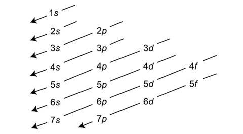
which of course was subsequently built into the topology of the periodic table.
Problem: Previously, both perturbation theory and the variational method were used to estimate the ground state energy of the helium atom. One can now ask: what about the \(1^{\text{st}}\) excited state?
Solution: From the perspective of \(H_0\), the \(1^{\text{st}}\) excited manifold has \(16\)-fold degeneracy; specifically, by applying the \(2\)-antisymmetrizer \(\sqrt{2}\mathcal A_2\) to any of the following, one obtains an \(H_0\)-eigenstate in the \(1^{\text{st}}\) excited subspace \(\text{ker}(H_0-E_21)\cap\bigwedge^2L^2(\mathbf R^3\to\mathbf C)\otimes\mathbf C^2\):
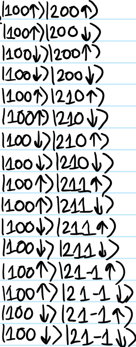
(aka Slater determinants). Even though this of course provides a basis for the \(16\)-dimensional space \(\text{ker}(H_0-E_21)\cap\bigwedge^2L^2(\mathbf R^3\to\mathbf C)\otimes\mathbf C^2\), some of these Slater determinants (e.g. \(\sqrt{2}\mathcal A_2|100\uparrow,200\downarrow\rangle\)) are not eigenstates of \(V\). Rather, because \([V,\mathbf L^2]=[V,L_z]=0\) is isotropic and \([V,\mathbf S^2]=[V,S_z]=0\) is furthermore spin-blind, where \(\mathbf L=\mathbf L_1+\mathbf L_2\) and \(\mathbf S=\mathbf S_1+\mathbf S_2\), it makes sense to instead work in an unentangled basis, specifically where each basis state factorizes into the product of a spatial wavefunction and a spinorial factor. This is achieved by the usual Clebsch-Gordan decomposition \((1/2)^{\otimes 2}=0\oplus 1\), and means that one should instead hybridize some of the Slater determinants:
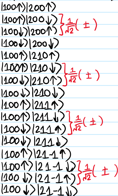
so that one is still left with \(16\) states at the end of the day, but now all of them are also simultaneous \((\mathbf S^2,S_3)\)-eigenstates. Now degenerate perturbation theory is very easy. Given \(|\Psi\rangle\in\biggr\{\frac{|100,200\rangle+|200,100\rangle}{\sqrt{2}}|0,0\rangle,\frac{|100,200\rangle-|200,100\rangle}{\sqrt{2}}|1,-1\rangle,…\biggr\}\) where the quantum numbers for \(\mathbf S^2,S_3\) are being used, because there are \(4\) different combinations of \((\ell,m_{\ell})=(0,0),(1,1),(1,0),(1,-1)\), one expects that to \(1^{\text{st}}\)-order the \(1^{\text{st}}\)-excited manifold’s \(16\)-fold degeneracy will decompose into \(4\) submanifolds each of \(4\)-fold degeneracy. Specifically:
\[\langle\Psi|V|\Psi\rangle=J\pm K\]
where \(J\) is called the direct energy and \(K\) the exchange energy (both are between \(2\)-particular \(|n\ell m_{\ell}\rangle\) states, and the \(+\) sign is taken if the spatial wavefunction is symmetric, while the \(-\) sign is taken if it’s antisymmetric). For example, for \(|\Psi\rangle=\frac{|100,211\rangle-|211,100\rangle}{\sqrt{2}}|1,1\rangle\), take the \(-\) sign with:
\[J_{100,211}=\langle 100,211|V|100,211\rangle=\alpha\hbar c\int d^3\mathbf x_1 d^3\mathbf x_2\frac{|\psi_{100}(\mathbf x_1)\psi_{211}(\mathbf x_2)|^2}{|\mathbf x_1-\mathbf x_2|}=\frac{59}{243}Z\alpha^2mc^2\]
\[K_{100,211}=\langle 100,211|V|211,100\rangle=\alpha\hbar c\int d^3\mathbf x_1 d^3\mathbf x_2\frac{\psi^{\dagger}_{100}(\mathbf x_1)\psi^{\dagger}_{211}(\mathbf x_2)\psi_{211}(\mathbf x_1)\psi_{100}(\mathbf x_2)}{|\mathbf x_1-\mathbf x_2|}=\frac{112}{6561}Z\alpha^2mc^2\]
And one indeed one can make an energy-splitting diagram that gives credence to the Aufbau rule (of course, the energy of all \(H_0\)-eigenstates increases with the electronic Coulomb repulsion \(V\)):
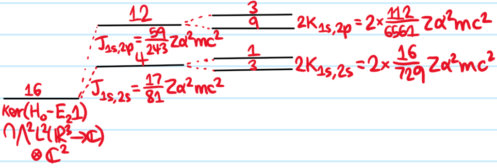
Note if one had instead used the Slater basis, ultimately one would still arrive at the same answer through having to find eigenvalues of block-diagonal matrices with blocks that look like \(\begin{pmatrix} J&-K\\-K&J\end{pmatrix}\).
(aside: a key selection rule \(\Delta s=0\) for \(\text E1\) transitions combined with the fact that \(s=0\) for the ground state means that starting in any \(s=1\) excited state would seem to be metastable…and indeed this is a forbidden transition, leading to a lifetime around \(\tau\approx 2.2^{\text h}\). Historically it was thought that \(s=0\) excited states corresponded to “parahelium” while \(s=1\) excited states corresponded to “orthohelium”).
Problem: After all the perturbation theory math in the above problem, what’s the key conceptual takeaway?
Solution: For unentangled states which may be factorized as the product of a spatial wavefunction and a spinorial component, when the spatial wavefunction is antisymmetric, the corresponding fermions are more likely to be found far from each other, and consequently the direct energy would be suppressed by this destructive quantum statistical interference (hence \(J-K\)). Conversely, symmetric spatial wavefunctions are enhanced by a sort of constructive quantum statistical interference (hence \(J+K\)).
Of course, one could also apply a variational approach just like was done for the ground state. This would confirm that electron screening is the key physics at play.
Problem: Show that for the Hartree product ansatz:
\[\Psi(\mathbf x_1,…,\mathbf x_N)=\psi_1(\mathbf x_1)…\psi_N(\mathbf x_N)\]
where \(\psi_1,…,\psi_N\) are \(N\) normalized single-particle wavefunctions, the expected energy \(\langle\Psi|H|\Psi\rangle\) with respect to the usual atomic Hamiltonian \(H\) is given by:
\[\langle\Psi|H|\Psi\rangle=-\frac{\hbar^2}{2m}\sum_{i=1}^N\int d^3\mathbf x\psi^{\dagger}_i(\mathbf x)\biggr|\frac{\partial}{\partial\mathbf x}\biggr|^2\psi_i(\mathbf x)-Z\alpha\hbar c\sum_{i=1}^N\int d^3\mathbf x\frac{|\psi_i(\mathbf x)|^2}{|\mathbf x|}\]
\[+\alpha\hbar c\sum_{1\leq i<j\leq N}\int d^3\mathbf x d^3\mathbf x’\frac{|\psi_i(\mathbf x)\psi_j(\mathbf x’)|^2}{|\mathbf x-\mathbf x’|}\]
(the last term is a sum over all pairs of direct energies \(J_{ij}\); there is no exchange energies \(K_{ij}\) yet because the Hartree ansatz \(|\Psi\rangle\) does not live in \(\bigwedge^N L^2(\mathbf R^3\to\mathbf C)\otimes\mathbf C^2\), indeed the ansatz doesn’t have any knowledge of the \(\mathbf C^2\) spinor! These deficiencies will be addressed later by the Hartree-Fock ansatz).
Solution: The key point about the Hartree product ansatz is that it’s separable, so just plug and separate integrals and remember that the \(\psi_i\) are normalized.
Problem: One would like to estimate the ground state wavefunction \(\Psi(\mathbf x_1,…,\mathbf x_N)\) of the \(N\)-electron atom within the Hartree framework (essentially mean-field theory). How can this be achieved?
Solution: By constrained minimization of the energy functional of \(\psi_1,…,\psi_N\):
\[\langle\Psi|H|\Psi\rangle-\sum_{i=1}^NE_i\left(\int d^3\mathbf x|\psi_i(\mathbf x)|^2-1\right)\]
where \(E_1,…,E_N\) are \(N\) Lagrange multipliers enforcing normalization constraints on the \(\psi_i\). Setting the functional derivative with respect to \(\psi^{\dagger}_i\) to zero is the quickest way to get the Schrodinger-equation like answer for each of the \(N\) single-particle wavefunctions \(\psi_i\):
\[\left(-\frac{\hbar^2}{2m}\biggr|\frac{\partial}{\partial\mathbf x}\biggr|^2-\frac{Z\alpha\hbar c}{|\mathbf x|}+V_i(\mathbf x)\right)\psi_i(\mathbf x)=E_i\psi_i(\mathbf x)\]
where:
\[V_i(\mathbf x)=\alpha\hbar c\sum_{j\neq i}\int d^3\mathbf x’\frac{|\psi_j(\mathbf x’)|^2}{|\mathbf x-\mathbf x’|}\]
is the Coulomb electrostatic potential energy experienced by the \(i^{\text{th}}\) electron due to the other \(N-1\) electrons (cf. the classical Coulomb electrostatic potential \(\phi(\mathbf x)=\frac{1}{4\pi\varepsilon_0}\int d^3\mathbf x’\frac{\rho(\mathbf x’)}{|\mathbf x-\mathbf x’|}\) with the charge density \(\rho(\mathbf x’)=-e|\psi(\mathbf x’)|^2\)). This system of \(N\) coupled nonlinear integrodifferential PDEs for \(\psi_1,…,\psi_N\) are also called the Hartree equations.
Problem: How are the Hartree equations solved numerically?
Solution: One can begin with a crude guess for the ground state \(\psi_i\) (such as the usual “Fermi sea” picture with hydrogenic atomic orbitals) and for each \(i=1,…,N\) obtain the interaction potential \(V_i(\mathbf x)\). Then, numerically solve the resulting \(i=1,…,N\) Schrodinger equations to obtain new \(\psi_i\), and repeat this process until hopefully it converges (this is also called the self-consistent field method).
Problem: Once these SCF iterations converges (hopefully) to some optimal set of \(N\) single-particle wavefunctions \(\psi^{\star}_i\), the corresponding Hartree estimate of the ground state wavefunction is of course \(\Psi^{\star}(\mathbf x_1,…,\mathbf x_N)=\psi^{\star}_1(\mathbf x_1)…\psi^{\star}_N(\mathbf x_N)\), but what about its corresponding ground state energy?
Solution: Although on the one hand this is just \(\langle\Psi^{\star}|H|\Psi^{\star}\rangle\), one can actually also write this in terms of the optimal Lagrange multipliers \(E^{\star}_i\), specifically because from the Hartree equations one can isolate:
\[E^{\star}_i=\int d^3\mathbf x\psi^{\star\dagger}_i(\mathbf x)\left(-\frac{\hbar^2}{2m}\biggr|\frac{\partial}{\partial\mathbf x}\biggr|^2-\frac{Z\alpha\hbar c}{|\mathbf x|}+V^{\star}_i(\mathbf x)\right)\psi^{\star}_i(\mathbf x)\]
So summing \(\sum_{i=1}^NE^{\star}_i\) would almost give \(\langle\Psi^{\star}|H|\Psi^{\star}\rangle\) except that it double-counts the direct energy term \(\sum_{i=1}^N\sum_{j\neq i}=2\sum_{1\leq i<j\leq N}\) so overall:
\[\langle\Psi^{\star}|H|\Psi^{\star}\rangle=\sum_{i=1}^NE^{\star}_i-\alpha\hbar c\sum_{1\leq i<j\leq N}\int d^3\mathbf x d^3\mathbf x’\frac{|\psi^{\star}_i(\mathbf x)\psi^{\star}_j(\mathbf x’)|^2}{|\mathbf x-\mathbf x’|}\]
(more precisely, since this is a variational estimate, the true ground state energy must be less than this).
Problem: Qualitatively, why is the ground state electron configuration of \(Z=19\) potassium \(\text K\) given by \(1s^22s^22p^63s^23p^64s^1\) rather than \(1s^22s^22p^63s^23p^63d^1\)?
Solution: Due to screening, a \(3d\) electron would have higher energy than a \(4s\) electron, so as far as the ground state is concerned, the latter is preferable. Hence, the Aufbau principle says \(4s\) is occupied before \(3d\). This can sort of be seen in the Hartree equations where, approximating \(V_i=V_i(r)\) as being approximately isotropic, one can define an effective nuclear charge \(Z_{\text{eff}}(r)\) such that the effective potential experienced by the \(i^{\text{th}}\) electron looks like:
\[-\frac{Z\alpha\hbar c}{r}+V_i(r)=-\frac{Z_{\text{eff}}(r)\alpha\hbar c}{r}\]
where \(\lim_{r\to 0}Z_{\text{eff}}(r)=Z=19\) and \(\lim_{r\to \infty}Z_{\text{eff}}(r)=1\)
Problem: The Hartree product ansatz \(\Psi(\mathbf x_1,…,\mathbf x_N)\) was purely a position space many-body wavefunction that did not involve any mention of spin (if it did, it would have canceled out in \(\langle\Psi|H|\Psi\rangle\) anyways because \(H\) is spin-blind). Even so, it didn’t live in \(\bigwedge^NL^2(\mathbf R^3\to\mathbf C)\). These deficiencies can be remedied via the Hartree-Fock ansatz, which is simply an antisymmetrization of the Hartree ansatz:
\[|\Psi\rangle=\sqrt{N!}\mathcal A_N|1\rangle\otimes…\otimes|N\rangle\]
where each single-particle spin-orbital \(\langle\mathbf x|i\rangle=\psi_i(\mathbf x)|\sigma\rangle\) with \(\sigma\in\{\uparrow,\downarrow\}\). It is often also written as a Slater determinant of the \(N\) single-particle spin-orbitals, but here the assignment of which electron occupies which single-particle spin-orbital \(|i\rangle\) is implicit in the ordering of the tensor product. Repeat everything from the Hartree derivation to derive the analogous Hartree-Fock equations.
Solution: One can show that, compared to the Hartree state, the expected energy of the Hartree-Fock state contains an additional (negative) exchange energy contribution for every pair of electrons with aligned spins \(\sigma_i=\sigma_j\):
\[\langle\Psi|H|\Psi\rangle=-\frac{\hbar^2}{2m}\sum_{i=1}^N\int d^3\mathbf x\psi^{\dagger}_i(\mathbf x)\biggr|\frac{\partial}{\partial\mathbf x}\biggr|^2\psi_i(\mathbf x)-Z\alpha\hbar c\sum_{i=1}^N\int d^3\mathbf x\frac{|\psi_i(\mathbf x)|^2}{|\mathbf x|}\]
\[+\alpha\hbar c\sum_{1\leq i<j\leq N}\int d^3\mathbf x d^3\mathbf x’\frac{|\psi_i(\mathbf x)\psi_j(\mathbf x’)|^2}{|\mathbf x-\mathbf x’|}-\alpha\hbar c\sum_{1\leq i<j\leq N}\delta_{\sigma_i\sigma_j}\int d^3\mathbf x d^3\mathbf x’\frac{\psi^{\dagger}_i(\mathbf x)\psi^{\dagger}_j(\mathbf x’)\psi_i(\mathbf x’)\psi_j(\mathbf x)}{|\mathbf x-\mathbf x’|}\]
(aside: the fact that the exchange energy lowers the total energy when spins are aligned means that the spins will prefer to align, and this is the essence of one of Hund’s rules).
Doing the constrained minimization again now yields the Hartree-Fock equations which are basically the Hartree equations with an additional non-local exchange potential:
\[\left(-\frac{\hbar^2}{2m}\biggr|\frac{\partial}{\partial\mathbf x}\biggr|^2-\frac{Z\alpha\hbar c}{|\mathbf x|}+V_{\text{int}}(\mathbf x)\right)\psi_i(\mathbf x)-\int d^3\mathbf x’ V_{\text{ex},i}(\mathbf x,\mathbf x’)\psi_i(\mathbf x’)=E_i\psi_i(\mathbf x)\]
but note that instead of \(\sum_{j\neq i}\), there is an apparent “self-energy” in the sum \(\sum_{j=1}^N\):
\[V_{\text{int}}(\mathbf x)=\alpha\hbar c\sum_{j=1}^N\int d^3\mathbf x’\frac{|\psi_j(\mathbf x’)|^2}{|\mathbf x-\mathbf x’|}\]
(so \(V_{\text{int}}\) is now the same for all electrons \(i=1,…,N\)). The self-energy is artificial though, and cancelled by a corresponding term from the exchange potential for each electron \(i\):
\[V_{\text{ex},i}(\mathbf x,\mathbf x’)=\alpha\hbar c\sum_{j=1}^N\delta_{\sigma_i\sigma_j}\int d^3\mathbf x’\frac{\psi^{\dagger}_j(\mathbf x’)\psi_j(\mathbf x)}{|\mathbf x-\mathbf x’|}\]
Problem: What is the key limitation of the Hartree-Fock method?
Solution: The fact that the Hartree-Fock ansatz only uses a single Slater determinant. Of course, the Hartree ansatz suffers from the same issue, but both in that it basically assumes that \(|\Psi\rangle\) is a non-interacting many-body state. In reality, the true ground state will of course be a superposition of Slater determinants, or in the \(2^{\text{nd}}\)-quantization view, a superposition of Fock states in the \(N\)-particle sector of the fermionic Fock space, and in that case the very language of “filling/occupying” shells/subshells which is familiar becomes unsuitable.