
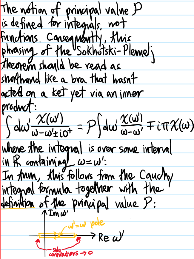
Problem: Prove the Sokhotski-Plemelj theorem on the real line \(\textbf R\):
\[\frac{1}{\omega-\omega’\pm i0^+}=\mathcal P\frac{1}{\omega-\omega’}\mp i\pi\delta(\omega-\omega’)\]
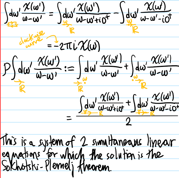
Solution: (in this solution, the function \(\chi(\omega)\) is assumed to be analytic on the integration interval in \(\textbf R\) to be able to apply the Cauchy integral formula):
Problem: Explain why any linear response function \(\chi\) should obey in the time domain \(\chi(t)=0\) for \(t<0\). Hence, what is the implication of this for \(\chi(\omega)\) in the frequency domain?
Solution: The fundamental definition of the linear response function \(\chi\) that gives it its name is that in the time domain \(\chi=\chi(t)\), the response \(x(t)\) should be proportional to the perturbation \(f(t)\) with \(\chi\) essentially acting as the proportionality constant according to the convolution:
\[x(t)=\int_{-\infty}^{\infty}dt’\chi(t-t’)f(t’)\]
(or equivalently the local behavior \(x(\omega)=\chi(\omega)f(\omega)\) in Fourier space). But if the “force” \(f(t’)\) is applied at time \(t’\), on causality grounds this can only affect the response \(x(t)\) at times \(t\geq t’\). In other words, it should be possible to change the limits on the integral from \(\int_{-\infty}^{\infty}dt’\) to \(\int_{-\infty}^tdt’\) without affecting the result. This therefore requires \(\chi(t-t’)=0\) for \(t<t’\), or more simply \(\chi(t)=0\) for \(t<0\). In light of this, \(\chi\) is also called a causal/retarded Green’s function.
Now then:
\[\chi(t)=\int_{-\infty}^{\infty}\frac{d\omega}{2\pi}e^{i\omega t}\chi(\omega)\]
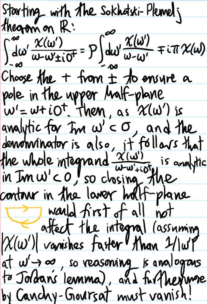
For \(t<0\), Jordan’s lemma asserts that one should close the contour in the lower half-plane \(\Im\omega<0\). But the fact that \(\chi(t)=0\) for \(t<0\) suggests that the sum of all residues of \(\chi(\omega)\) in the lower half-plane \(\Im\omega<0\) should be “traceless”. A sufficient condition for this is if \(\chi(\omega)\) is analytic in the lower half-plane \(\Im\omega<0\), and henceforth this will be assumed.
Problem: Qualitatively, what do the Kramers-Kronig relations assert? What about quantitatively?
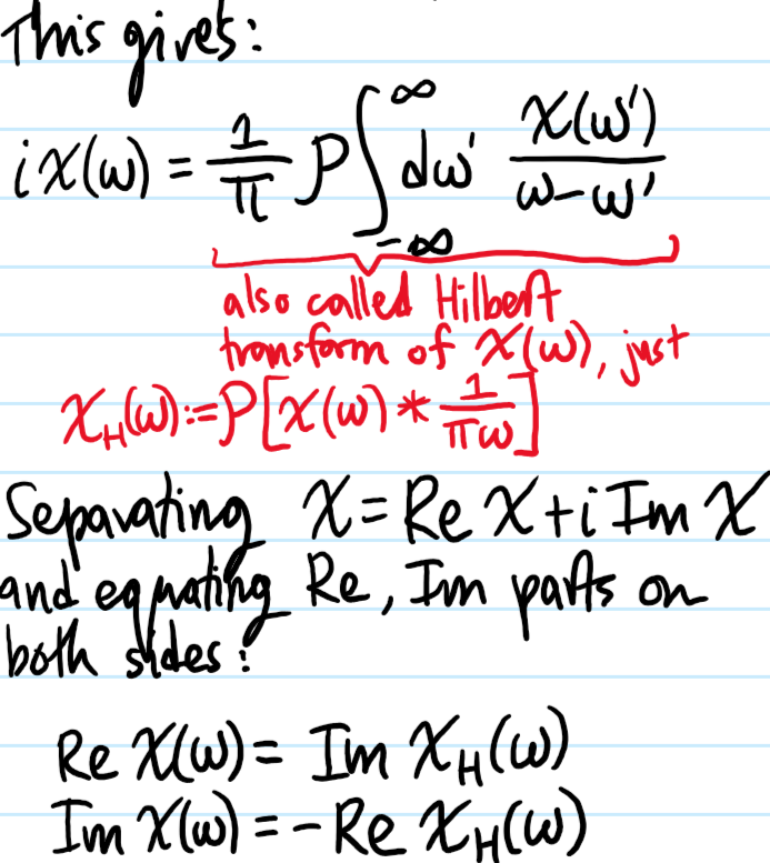
Solution: Qualitatively, for a linear response function like \(\chi(\omega)\) which is analytic in the lower half-plane \(\Im\omega<0\), knowing its reactive part \(\Re\chi(\omega)\) is equivalent to knowing its absorptive/dissipative spectrum \(\Im\chi(\omega)\) which in turn is equivalent to knowing \(\chi(\omega)\) itself.
\[\Re\chi(\omega)\Leftrightarrow\Im\chi(\omega)\Leftrightarrow\chi(\omega)\]
Quantitatively, the bridges \(\Leftrightarrow\) are provided by the Kramers-Kronig relations:
Note: sometimes the discussion of Kramers-Kronig relations are phrased in terms of \(\chi(\omega)\) being analytic in the upper half-plane. This stems from an unconventional definition of the Fourier transform \(\chi(t)=\int_{-\infty}^{\infty}\frac{d\omega}{2\pi}e^{-i\omega t}\chi(\omega)\) rather than the more conventional definition \(\chi(t)=\int_{-\infty}^{\infty}\frac{d\omega}{2\pi}e^{i\omega t}\chi(\omega)\) used above. Consequently, the minus signs in the Kramers-Kronig relations may also appear flipped around.
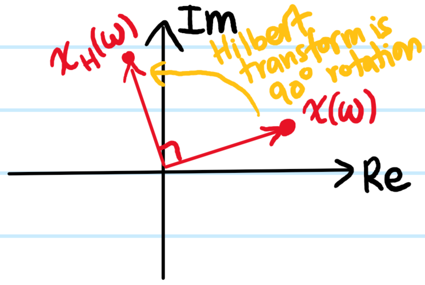
Problem: If the response \(x(t)\) and the driving force \(f(t)\) are both real-valued, what are the implications of this for \(\Re\chi(\omega)\) and \(\Im\chi(\omega)\)?
Solution: Then \(\chi(t)\in\textbf R\) must also be real-valued, so \(\chi(\omega)\) is Hermitian:
\[\chi^{\dagger}(\omega)=\chi(-\omega)\]
Consequently, the reactive response \(\Re\chi(-\omega)=\Re\chi(\omega)\) is even while the absorptive/dissipative response \(\Im\chi(-\omega)=-\Im\chi(\omega)\) is odd.
Problem: State the thermodynamic sum rule.
Solution: The sum rule asserts that if one knows how much a system absorbs/dissipates at all frequencies \(\omega\in\textbf R\), then one can deduce the system’s DC linear response \(\chi(\omega=0)\), called its susceptibility (of course the Kramers-Kronig relations actually show that knowing \(\Im\chi(\omega)\) allows complete reconstruction of \(\chi(\omega)\) at all frequencies \(\omega\in\textbf R\), not just \(\omega=0\)).
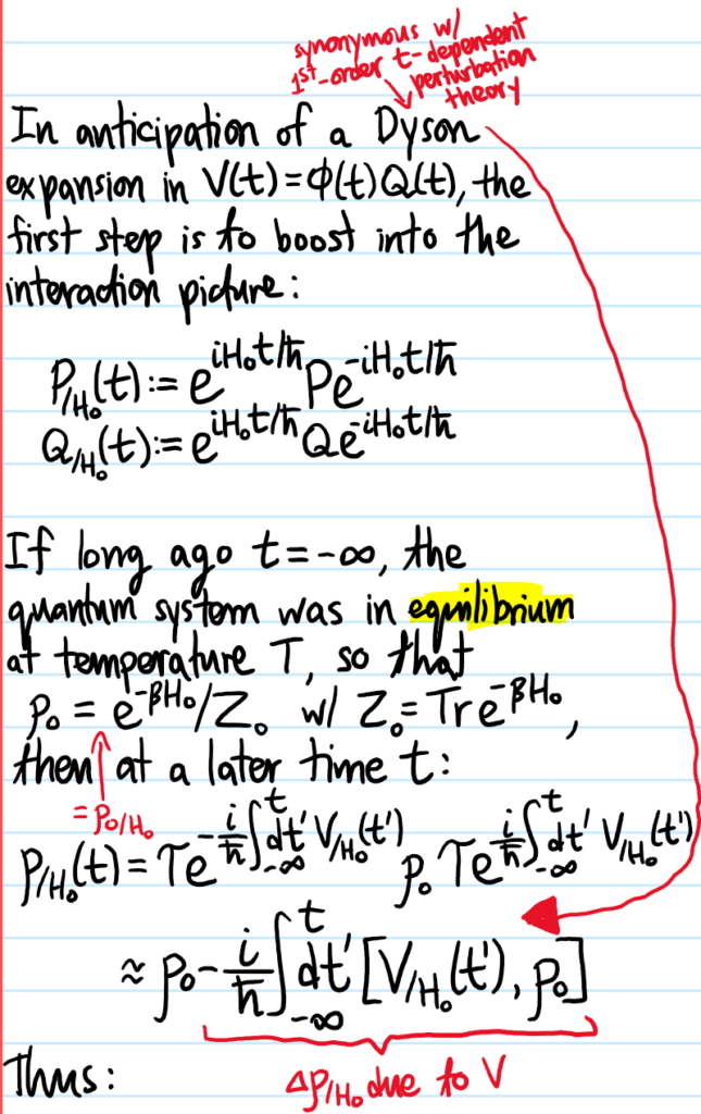
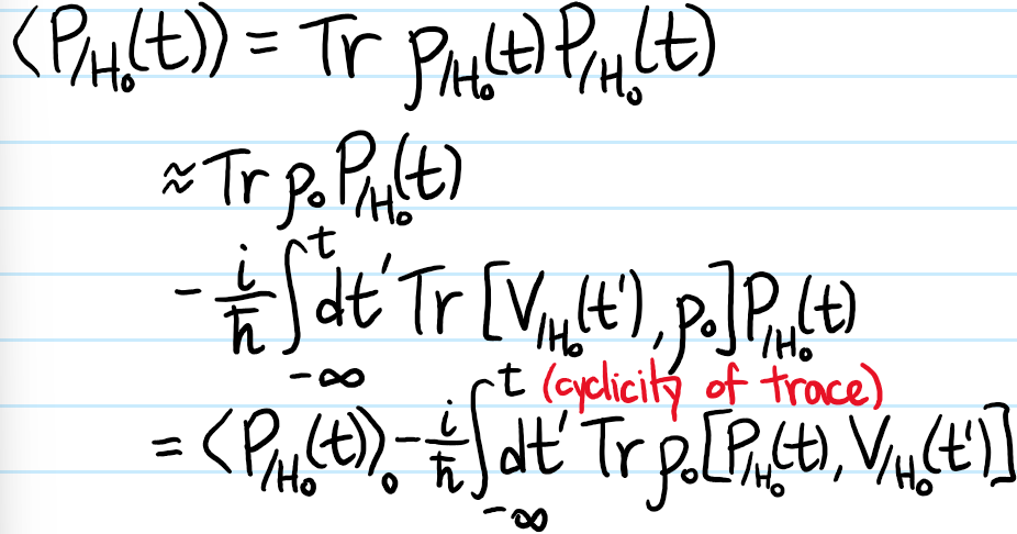
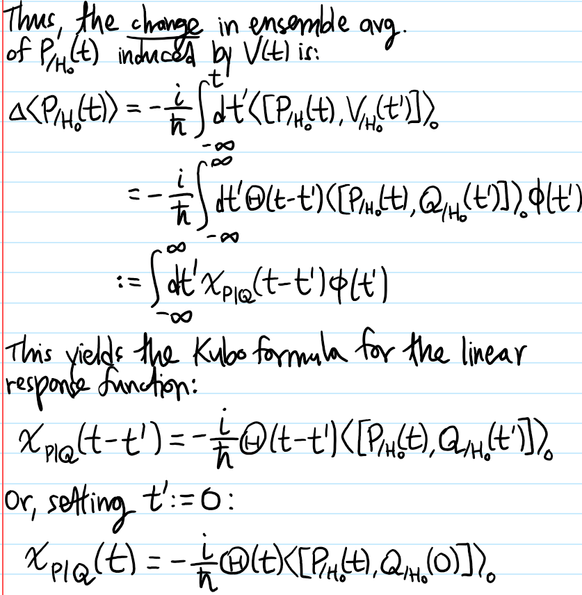
Problem: Given a \(t\)-dependent Legendre perturbation of the form \(V(t)=\phi(t)Q\) where \(Q\) is a (possibly also \(t\)-dependent) operator and \(\phi(t)\) is scalar-valued, define the linear response function \(\chi_{P|Q}(t)\) of another operator \(P\) due to \(Q\) and show that within the framework of linear response theory it is given by Kubo’s formula:
\[\chi_{P|Q}(t)=-\frac{i}{\hbar}\Theta(t)\langle[P_{/H_0}(t),Q_{/H_0}(0)]\rangle_0\]
Solution:
Problem: Prove the fluctuation-dissipation theorem: