
Problem: In a multilayer perceptron (MLP), how are layers conventionally counted?
Solution: The input layer \(\textbf x\equiv\textbf a^{(0)}\) is also called “layer \(0\)”. However, if someone says that an MLP has e.g. \(7\) layers, what this means is that in fact it has \(6\) hidden layers \(\textbf a^{(1)},\textbf a^{(2)},…,\textbf a^{(6)}\), together with the output layer \(\textbf a^{(7)}\). In other words, the input layer \(\textbf a^{(0)}\) is not counted by convention.
Problem: Write down the formula for the activation \(a^{(\ell)}_n\) of the \(n^{\text{th}}\) neuron in the \(\ell^{\text{th}}\) layer of a multilayer perceptron (MLP) artificial neural network.
Solution: Using a sigmoid activation function, the activation of the \(n^{\text{th}}\) neuron in the \(\ell^{\text{th}}\) layer is:
\[a^{(\ell)}_n=\frac{1}{e^{-(\textbf w^{(\ell)}_n\cdot\textbf a^{(\ell-1)}+b^{(\ell)}_n)}+1}\]
Problem: What is the output from the following Python code?
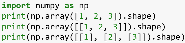
Solution: The first NumPy array has shape \((3,)\). The second NumPy array has shape \((1,3)\). The third NumPy array has shape \((3,1)\). While this may seem like a trivial distinction, in fact it’s very important when it comes to using the TensorFlow library, which only accepts matrices of the latter \(2\) kind.
Problem: What type of activation function is most often used for the hidden layers of an MLP? What about for the output layer?
Solution: The most common activation function for the hidden layers is the ReLU (rectified linear unit), defined as \(a_{\text{ReLU}}(x):=\text{max}(0,x)\) whereas the activation function used for the output layer depends on the range of target labels \(y\) (i.e. if it’s about binary classification \(y\in\{0,1\}\) then a sigmoid activation would be useful, if it’s \(y\in[0,\infty)\) then another ReLU would be useful, and if it’s \(y\in\textbf R\) then a linear activation function, would be useful; there are also other more exotic activation functions possible).
There are \(2\) reasons for using ReLU (rather than the historical sigmoid functions). The first (less important) reason is that ReLU is clearly a bit faster to compute than a sigmoid. The second (more important) reason is that experimentally one finds \(\partial/\partial(W,\textbf b)\)-descent is faster with ReLU than with sigmoids (intuitively this is due to the presence of more “flat” sections on the graph of the sigmoid than the ReLU).
Naturally one might also ask “why not just linear activations all the way through”? The reason is because this would just reduce to linear regression (i.e. the neural network wouldn’t buy one anything new). Similarly, changing the activation of the output layer to a sigmoid while keeping the hidden layers as linear activations just reduces to logistic classification.
Problem: Import the subset of training examples in the MNIST database whose target value is either \(y=0\) or \(y=1\), and train a multilayer perceptron with \(3\) hidden layers \((N_1,N_2,N_3)=(25,15,1)\) to do logistic binary classification on this subset (and evaluate the accuracy, and for fun have a look at the misclassified images).
Solution:
import tensorflow as tf
# Load the MNIST dataset
(x_train, y_train), (x_test, y_test) = tf.keras.datasets.mnist.load_data()

print(x_train.shape)  # (60000, 28, 28)
print(y_train.shape) # (60000,)
(60000, 28, 28)
(60000,)
import matplotlib.pyplot as plt
import numpy as np

plt.figure(figsize=(15, 15))
for n in np.arange(5):
    plt.subplot(2, 5, n+1)
    plt.imshow(x_train[n, :, :], cmap='gray')
    plt.title(f"Target Label: {y_train[n]}")

# Get only the subset of training examples in the MNIST database whose target label is either 0 or 1
subset_Boolean = (y_train < 2)
x_train_01_only = x_train[subset_Boolean, :, :]
x_train_01_only.shape #(12665, 28, 28)
y_train_01_only = y_train[subset_Boolean]
y_train_01_only.shape #(12665,)

# Reshape to (60000, 28*28) to be compatible with TensorFlow MLP.fit later
x_train_01_only_reshaped = x_train_01_only.reshape(x_train_01_only.shape[0], -1)
plt.figure(figsize=(15, 15))
for n in np.arange(5):
    plt.subplot(2, 5, n+1)
    plt.imshow(x_train_01_only[n, :], cmap='gray')
    plt.title(f"Target Label: {y_train_01_only[n]}")

from tensorflow.keras.layers import Dense
from tensorflow.keras.models import Sequential

MLP = Sequential([tf.keras.Input(shape=(784,)),
                  Dense(units=25, activation='relu'),
                 Dense(units=15, activation='relu'),
                 Dense(units=1, activation='sigmoid')])

MLP.compile(loss=tf.keras.losses.BinaryCrossentropy())
MLP.fit(x_train_01_only_reshaped, y_train_01_only, epochs=50)
Epoch 1/50
396/396 ━━━━━━━━━━━━━━━━━━━━ 2s 2ms/step - loss: 0.5120
Epoch 2/50
396/396 ━━━━━━━━━━━━━━━━━━━━ 1s 2ms/step - loss: 0.0361
Epoch 3/50
396/396 ━━━━━━━━━━━━━━━━━━━━ 1s 2ms/step - loss: 0.0111
Epoch 4/50
396/396 ━━━━━━━━━━━━━━━━━━━━ 1s 2ms/step - loss: 0.0286
Epoch 5/50
396/396 ━━━━━━━━━━━━━━━━━━━━ 1s 2ms/step - loss: 0.0127
Epoch 6/50
396/396 ━━━━━━━━━━━━━━━━━━━━ 1s 2ms/step - loss: 0.0142
Epoch 7/50
396/396 ━━━━━━━━━━━━━━━━━━━━ 1s 2ms/step - loss: 0.0049
Epoch 8/50
396/396 ━━━━━━━━━━━━━━━━━━━━ 1s 2ms/step - loss: 0.0040
Epoch 9/50
396/396 ━━━━━━━━━━━━━━━━━━━━ 1s 2ms/step - loss: 2.5909e-05
Epoch 10/50
396/396 ━━━━━━━━━━━━━━━━━━━━ 1s 2ms/step - loss: 0.0028
Epoch 11/50
396/396 ━━━━━━━━━━━━━━━━━━━━ 1s 2ms/step - loss: 2.8652e-04
Epoch 12/50
396/396 ━━━━━━━━━━━━━━━━━━━━ 1s 2ms/step - loss: 4.5746e-04
Epoch 13/50
396/396 ━━━━━━━━━━━━━━━━━━━━ 1s 2ms/step - loss: 0.0014
Epoch 14/50
396/396 ━━━━━━━━━━━━━━━━━━━━ 1s 2ms/step - loss: 3.9976e-07
Epoch 15/50
396/396 ━━━━━━━━━━━━━━━━━━━━ 1s 2ms/step - loss: 1.5654e-04
Epoch 16/50
396/396 ━━━━━━━━━━━━━━━━━━━━ 1s 2ms/step - loss: 2.5585e-09
Epoch 17/50
396/396 ━━━━━━━━━━━━━━━━━━━━ 1s 2ms/step - loss: 2.1332e-10
Epoch 18/50
396/396 ━━━━━━━━━━━━━━━━━━━━ 1s 2ms/step - loss: 7.2755e-10
Epoch 19/50
396/396 ━━━━━━━━━━━━━━━━━━━━ 1s 2ms/step - loss: 2.4617e-10
Epoch 20/50
396/396 ━━━━━━━━━━━━━━━━━━━━ 1s 2ms/step - loss: 9.2963e-11
Epoch 21/50
396/396 ━━━━━━━━━━━━━━━━━━━━ 1s 2ms/step - loss: 1.4893e-10
Epoch 22/50
396/396 ━━━━━━━━━━━━━━━━━━━━ 1s 2ms/step - loss: 8.3827e-11
Epoch 23/50
396/396 ━━━━━━━━━━━━━━━━━━━━ 1s 2ms/step - loss: 3.9026e-10
Epoch 24/50
396/396 ━━━━━━━━━━━━━━━━━━━━ 1s 2ms/step - loss: 2.0069e-10
Epoch 25/50
396/396 ━━━━━━━━━━━━━━━━━━━━ 1s 2ms/step - loss: 5.2177e-11
Epoch 26/50
396/396 ━━━━━━━━━━━━━━━━━━━━ 1s 2ms/step - loss: 2.4525e-10
Epoch 27/50
396/396 ━━━━━━━━━━━━━━━━━━━━ 1s 2ms/step - loss: 1.4602e-10
Epoch 28/50
396/396 ━━━━━━━━━━━━━━━━━━━━ 1s 2ms/step - loss: 3.3851e-11
Epoch 29/50
396/396 ━━━━━━━━━━━━━━━━━━━━ 1s 2ms/step - loss: 3.2089e-11
Epoch 30/50
396/396 ━━━━━━━━━━━━━━━━━━━━ 1s 2ms/step - loss: 2.7352e-11
Epoch 31/50
396/396 ━━━━━━━━━━━━━━━━━━━━ 1s 2ms/step - loss: 7.5922e-11
Epoch 32/50
396/396 ━━━━━━━━━━━━━━━━━━━━ 1s 2ms/step - loss: 2.9092e-11
Epoch 33/50
396/396 ━━━━━━━━━━━━━━━━━━━━ 1s 2ms/step - loss: 8.3690e-11
Epoch 34/50
396/396 ━━━━━━━━━━━━━━━━━━━━ 1s 2ms/step - loss: 1.4150e-11
Epoch 35/50
396/396 ━━━━━━━━━━━━━━━━━━━━ 1s 2ms/step - loss: 4.1584e-11
Epoch 36/50
396/396 ━━━━━━━━━━━━━━━━━━━━ 1s 2ms/step - loss: 8.3697e-11
Epoch 37/50
396/396 ━━━━━━━━━━━━━━━━━━━━ 1s 2ms/step - loss: 2.1891e-11
Epoch 38/50
396/396 ━━━━━━━━━━━━━━━━━━━━ 1s 2ms/step - loss: 6.1118e-11
Epoch 39/50
396/396 ━━━━━━━━━━━━━━━━━━━━ 1s 2ms/step - loss: 1.7206e-11
Epoch 40/50
396/396 ━━━━━━━━━━━━━━━━━━━━ 1s 2ms/step - loss: 6.9571e-11
Epoch 41/50
396/396 ━━━━━━━━━━━━━━━━━━━━ 1s 2ms/step - loss: 4.1679e-11
Epoch 42/50
396/396 ━━━━━━━━━━━━━━━━━━━━ 1s 2ms/step - loss: 2.2382e-11
Epoch 43/50
396/396 ━━━━━━━━━━━━━━━━━━━━ 1s 2ms/step - loss: 1.8092e-11
Epoch 44/50
396/396 ━━━━━━━━━━━━━━━━━━━━ 1s 2ms/step - loss: 4.7662e-11
Epoch 45/50
396/396 ━━━━━━━━━━━━━━━━━━━━ 1s 2ms/step - loss: 3.0981e-11
Epoch 46/50
396/396 ━━━━━━━━━━━━━━━━━━━━ 1s 2ms/step - loss: 5.3414e-11
Epoch 47/50
396/396 ━━━━━━━━━━━━━━━━━━━━ 1s 2ms/step - loss: 6.5965e-11
Epoch 48/50
396/396 ━━━━━━━━━━━━━━━━━━━━ 1s 2ms/step - loss: 2.8171e-11
Epoch 49/50
396/396 ━━━━━━━━━━━━━━━━━━━━ 1s 2ms/step - loss: 3.7733e-11
Epoch 50/50
396/396 ━━━━━━━━━━━━━━━━━━━━ 1s 2ms/step - loss: 1.4982e-11
<keras.src.callbacks.history.History at 0x25370d10350>
# Some testing examples (TESTING = NOT TRAINING!)
plt.figure(figsize=(15, 15))
for n in np.arange(5):
    plt.subplot(2, 5, n+1)
    plt.imshow(x_test[n, :, :], cmap='gray')
    plt.title(f"Target Label: {y_test[n]}")

subset_Boolean = (y_test < 2)
x_test_01_only = x_test[subset_Boolean, :, :]
x_test_01_only.shape #(2115, 28, 28)
y_test_01_only = y_test[subset_Boolean]
y_test_01_only.shape #(2115,)

# Reshape to (60000, 28*28) to be compatible with TensorFlow MLP.fit later
x_test_01_only_reshaped = x_test_01_only.reshape(x_test_01_only.shape[0], -1)
plt.figure(figsize=(15, 15))
for n in np.arange(5):
    plt.subplot(2, 5, n+1)
    plt.imshow(x_test_01_only[n, :], cmap='gray')
    plt.title(f"Target Label: {y_test_01_only[n]}")

y_hat = MLP.predict(x_test_01_only_reshaped)
y_hat_reshaped = y_hat.reshape(y_test_01_only.shape[0])
y_hat_reshaped_int = np.round(y_hat_reshaped)
accuracy = (y_hat_reshaped_int == y_test_01_only).mean()
print(f"MLP Binary Classification Accuracy: {accuracy:.4f}")
67/67 ━━━━━━━━━━━━━━━━━━━━ 0s 3ms/step
MLP Binary Classification Accuracy: 0.9995
probs = MLP.predict(x_test_01_only_reshaped)   # shape (N, 1)
y_hat = (probs>=0.5).astype(int).reshape(-1)               # shape (N,), can also use .ravel()
accuracy = (y_hat==y_test_01_only).mean()
print(f"MLP Binary Classification Accuracy: {accuracy:.4f}")
67/67 ━━━━━━━━━━━━━━━━━━━━ 0s 2ms/step
MLP Binary Classification Accuracy: 0.9995
# Which one was misclassified?
deviation_Booleans = (y_hat != y_test_01_only)

x_test_01_only_deviations = x_test_01_only[deviation_Booleans]
y_test_01_only_deviations = y_test_01_only[deviation_Booleans]
len(x_test_01_only_deviations) #4

plt.figure(figsize=(20, 15))
for i, test_x in enumerate(x_test_01_only_deviations):
    plt.subplot(2, 5, i+1)
    plt.imshow(test_x, cmap='gray')
    plt.title(f"Target Label: {y_test_01_only_deviations[i]}, MLP Prediction: {y_hat[deviation_Booleans][i]}")

Problem: Write down the activations of a softmax output layer with \(N_{\text{out}}\) neurons to be used for multiclass classification with \(N_{\text{out}}\) classes.
Solution: For \(1\leq n\leq N_{\text{out}}\), define the conventional variables \(z_n:=\textbf w_n\cdot\textbf x+b_n\), where \(\textbf w_n,b_n\) are the weights and bias of the \(n^{\text{th}}\) neuron in that \(N_{\text{out}}\)-neuron output layer, and \(\textbf x\) here represents the activation vector of the previous (hidden) layer of neurons. Then the softmax activation of the \(n^{\text{th}}\) neuron in that output layer is given by:
\[a^{\text{softmax}}_n(z_1,…,z_N):=\frac{e^{z_n}}{e^{z_1}+…+e^{z_N}}\]
This has the interpretation of a Boltzmann-like probability distribution over the \(N\) classes because:
\[\sum_{n=1}^Na^{\text{softmax}}_n(z_1,…,z_N)=1\]
Problem: What is the corresponding loss function for softmax classification?
Solution: If the target label \(y=n\):
\[L(a^{\text{softmax}}_n)=-\ln a^{\text{softmax}}_n\]
which is the usual definition of information content.
Problem: Explain why softmax classification is a generalization of logistic classification.
Problem: Suppose one is deciding between several possible neural network architectures. One has a bunch of data \(\mathcal D:=\{(\textbf x_i,y_i)\}\) on one’s hands. What is a quantitative way to perform model selection in this case (i.e. decide which neural network architecture to use)?
Solution: First, randomly partition the data set \(\mathcal D\) into \(3\) disjoint subsets \(\mathcal D=\mathcal D_{\text{tr}}\cup\mathcal D_{\text{cv}}\cup\mathcal D_{\text{te}}\), viz. a training subset \(\mathcal D_{\text{tr}}\), a cross-validation subset \(\mathcal D_{\text{cv}}\), and a testing subset \(\mathcal D_{\text{te}}\); note as a rule of thumb the size of these subsets in relation to the original data set should be around \(\#\mathcal D_{\text{tr}}/\#\mathcal D\approx 60\%\) and \(\#\mathcal D_{\text{cv}}/\#\mathcal D\approx \#\mathcal D_{\text{te}}/\#\mathcal D\approx 20\%\). Then, each of these \(3\) subsets plays its respective role for each of the \(3\) steps:
- For each neural network architecture, minimize \(C_{\mathcal D_{\text{tr}}}(\{\textbf w_n^{(\ell)}\},\{b_n^{(\ell)}\}|\lambda=0)\), thereby obtaining a set of optimal weights \(\{\textbf w_n^{(\ell)*}\}\) and optimal biases \(\{b_n^{(\ell)*}\}\) for the neurons in that particular neural network architecture.
- For each neural network architecture, using its optimal \(\{\textbf w_n^{(\ell)}\},\{b_n^{(\ell)}\}\) from step \(1\), evaluate \(C_{\mathcal D_{\text{cv}}}(\{\textbf w_n^{(\ell)*}\},\{b_n^{(\ell)*}\}|\lambda=0)\). The neural network one should choose is then the one for which this cross-validation error is the minimum.
- (Optional) An unbiased estimator for that neural network’s generalization error is then given by \(C_{\mathcal D_{\text{te}}}(\{\textbf w_n^{(\ell)*}\},\{b_n^{(\ell)*}\}|\lambda=0)\). This is unbiased because neither the particular neural network architecture nor its weights and biases were determined from \(\mathcal D_{\text{te}}\).
Problem: Explain the difference between a model’s representational capacity and its effective capacity.
Solution: The representational capacity of a model is essentially asking about how many possible functions can be reached by the ansatz. For example, a quadratic model \(\hat y(x|w_1,w_2,b)=w_1x^2+w_2x+b\) clearly has greater representational capacity than the linear model \(\hat y(x|w,b)=wx+b\) because the function space spanned by the latter is a subset of the function space spanned by the former. In practice, the true representational capacity of a model may be difficult to exploit due to the nonconvex optimization landscape. Taking this limitation into account yields the concept of an effective capacity which is always less than or equal to the model’s representational capacity.
Problem: For a binary classifier, explain how the Vapnik-Chervonenkis (VC) dimension \(\dim_{\text{VC}}\) provides an integer proxy for its representational capacity.
Solution: One can first define a slightly more general concept of VC dimension \(\dim_{\text{VC}}\) for any arbitrary collection \(\mathcal C\) of sets.
A collection of sets \(\mathcal C\) is said to shatter a set \(X\) iff every subset of \(X\) can be “carved out” by taking \(X\) and intersecting it with some set in \(\mathcal C\); this is equivalent to saying that the power set \(2^X=\mathcal C\cap X\) where \(\mathcal C\cap X\) is defined in the obvious manner.
The VC dimension \(\dim_{\text{VC}}\) of the collection \(\mathcal C\) of sets is then defined to the cardinality of the largest set \(X\) which can be shattered by \(\mathcal C\).
The way this applies to a binary classifier is that because a binary classifier works by taking feature space (e.g. \(\mathbf R^n\)) and dividing it up into \(2\) disjoint regions (such that features on one side of the boundary are classified \(0\) while features on the other side are classified \(1\)), \(\mathcal C\) is taken to be the collection of all such regions that can be classified as e.g. \(1\) for instance. Then \(X\) is simply the collection of feature vectors in that feature space (e.g. \(\mathbf R^n\)).
For example, the classic XOR counterexample provides an intuition for why the VC dimension of any linear binary classifier in the plane \(\mathbf R^2\) is \(\dim_{\text{VC}}=3\) (and in fact more generally the VC dimension of a linear binary classifier is \(\dim_{\text{VC}}=n+1\) in \(\mathbf R^n\)).
Problem: Show that the mean-squared error (MSE) admits a decomposition into \(3\) non-negative terms of the form:
\[\text{MSE}=\text{Bias}^2+\text{Variance}+\text{Bayes Error}\]
and give expressions for all \(4\) terms in this equation. Using this identity, explain the bias-variance tradeoff.
Solution: The mean squared error of a point estimator \(\hat y=\hat y(x)\) for an underlying random variable \(y=y(x)\) is in this case a proxy for generalization error:
\[\text{MSE}:=\langle (\hat y-y)^2\rangle\]
The bias of the point estimator \(\hat y\) is:
\[\text{Bias}:=\langle\hat y\rangle-\langle y\rangle\]
The variance of the point estimator \(\hat y\) is:
\[\text{Variance}:=\langle (\hat y-\langle\hat y\rangle)^2\rangle\]
The Bayes error is an irreducible error associated with the random-variable nature of \(y\) itself rather than the model \(\hat y\) (e.g. \(2\) houses with the exact same features selling for different prices in a regression model, or \(2\) emails with identical features but one is spam and another isn’t in a classification model):
\[\text{Bayes error}=\sigma^2_y\]
(aside: the reason this is called a Bayes error is that \(y\) is being treated as a random variable rather than how a frequentist would view \(y\) as a fixed parameter…clearly if \(y\) were simply fixed then there would be no variance \(\sigma^2_y=0\) and hence no Bayes error).
Since the Bayes error is generally not in one’s control, it follows that the best one can in principle hope for is \(\text{MSE}=\text{Bayes error}\), so this begs the question of how one can minimize the sum of \(\text{Bias}^2+\text{Variance}\)? Here, the dilemma of the bias-variance tradeoff is observed, namely \(\text{Bias}^2\) tends to be an decreasing function of the model’s effective capacity whereas \(\text{Variance}\) tends to be an increasing function of the effective capacity of \(\hat y\):
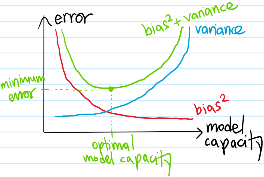
The challenge is thus to find that sweet spot in model capacity (also called model complexity/flexibility, etc.) that minimizes the sum \(\text{Bias}^2+\text{Variance}\) of these \(2\) errors as much as possible, since that’s all one has control over. If the model capacity is less than this optimal capacity, then one would be in a high-bias, low-variance regime of underfitting. By contrast, if the model capacity exceeds the optimal model capacity, then this low-bias, high-variance regime would be at risk of overfitting.
Practically, one can use as a proxy for diagnosis:
\[\text{Bias}^2\sim C_{\mathcal D_{\text{train}}}(\{\textbf w_n^{(\ell)*}\},\{b_n^{(\ell)*}\}|\lambda=0)-C_0\]
\[\text{Variance}\sim C_{\mathcal D_{\text{cv}}}(\{\textbf w_n^{(\ell)*}\},\{b_n^{(\ell)*}\}|\lambda=0)-C_{\mathcal D_{\text{train}}}(\{\textbf w_n^{(\ell)*}\},\{b_n^{(\ell)*}\}|\lambda=0)\]
where \(C_0\) is some notion of “baseline cost” (e.g. human performance).
Problem: The previous problem explained how to diagnose high bias or high variance in a neural network model. Once they have been diagnosed, what’s the cure?
Solution: Essentially there are \(2\) axes over which one has control:
- Add more training examples if the neural network is diagnosed with high variance (reducing training examples is never a good idea).
- Feature engineering/regularization: if the neural network is diagnosed with high bias (aka underfitting) then more features might help. By contrast, if diagnosed with high variance (aka overfitting), then fewer features might help. An equivalent way to filter out features is with regularization (e.g. increasing \(\lambda\) is isomorphic to removing features, and vice versa).
Problem: Draw a flow chart to illustrate a typical machine learning workflow:
Solution: It almost never hurts to go to a bigger neural network as long as one regularizes appropriately:
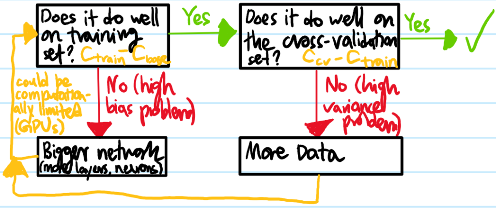
(bigger network = more features)
Problem: Explain the meaning of the phrase “large neural networks are low-bias machines“.
Solution: Loosely speaking, provided:
\[\text{Number of Neurons in Neural Network}\gg\#\mathcal D\]
then neural networks can almost always fit the training data pretty well, meaning low-bias. As a result, it is typically the case that high-variance is a bigger problem.
Problem: Describe what error analysis means in the context of evaluating a machine learning system’s classification performance (does it also apply to regression?)
Solution: The idea is that, if a neural network is diagnosed with high variance issues, rather than just feeding it more random training examples, one should feed it in a smarter way by first looking at the exact nature of the misclassifications.
Problem: Suppose a neural network is diagnosed with high variance, and error analysis shows that in fact one simply needs more training examples in general, but new training examples are scarce; in this case, what are \(2\) additional techniques one can try to improve the performance of one’s ML system?
Solution:
- Data Augmentation: take existing training examples one already has, and perturb them in “representative” ways so as to obtain new training examples.
- Data Synthesis: create new “representative” training examples out of thin air. There are many ways to do this depending on the specific application.
Problem: What are the \(2\) steps of transfer learning?
Solution:
- Supervised Pretraining: train a neural network on a loosely related task.
- Fine Tuning: taking the weights and biases of the hidden layers in the pretrained neural network as a starting point, do further training on either just the output layer or of the entire neural network, until it performs as desired on the task for which abundant data was not so immediately available.