
Gross Structure of Hydrogenic Atoms
In non-relativistic quantum mechanics, the gross structure Hamiltonian \(H_{\text{gross}}\) for a hydrogenic atom \(N^{Z+}\cup e^-\) consisting of a single electron \(e^-\) in a bound state with an atomic nucleus \(N^{Z+}\) of nuclear charge \(Z\in\textbf Z^+\) is:
\[H_{\text{gross}}=\frac{\textbf P^2_{N^{Z+}}}{2m_{N^{Z+}}}\otimes 1_{e^-}+ 1_{N^{Z+}}\otimes\frac{\textbf P^2_{e^-}}{2m_{e^-}}-\frac{Z\alpha\hbar c}{|1_{N^{Z+}}\otimes\textbf X_{e^-}-\textbf X_{N^{Z+}}\otimes 1_{e^-}|}\]
where the state space is comprised of \(\mathcal H=\mathcal H_{N^{Z+}}\otimes\mathcal H_{e^-}\). However, since this is just a \(2\)-body problem, one can also take the view that \(\mathcal H=\mathcal H_{\text{CoM}}\otimes\mathcal H_{\text{rel}}\).
Hence, defining the operators:
\[\textbf P_{\text{CoM}}\otimes 1_{\text{rel}}:=\textbf P_{N}\otimes 1_{e^-}+1_{N^{Z+}}\otimes\textbf P_{e^-}\]
\[1_{\text{CoM}}\otimes\textbf X_{\text{rel}}:=1_{N^{Z+}}\otimes\textbf X_{e^-}-\textbf X_{N^{Z+}}\otimes 1_{e^-}\]
\[1_{\text{CoM}}\otimes\textbf P_{\text{rel}}=(m_{N^{Z+}}1_{N^{Z+}}\otimes\textbf P_{e^-}-m_{e^-}\textbf P_{N^{Z+}}\otimes 1_{e^-})/M\]
the gross structure Hamiltonian becomes:
\[H_{\text {gross}}=\frac{\textbf P^2_{\text{CoM}}}{2M}\otimes 1_{\text{rel}}+1_{\text{CoM}}\otimes\frac{\textbf P^2_{\text{rel}}}{2\mu}-\frac{Z\alpha\hbar c}{|1_{\text{CoM}}\otimes\textbf X_{\text{rel}}|}\]
where the hydrogenic atom’s total mass is \(M=m_{N^{Z+}}+m_{e^-}\) whereas its reduced mass is \(\mu=m_{N^{Z+}}m_{e^-}/M\). In what follows, it will also be helpful to imagine factoring out the CoM identity operator \(1_{\text{CoM}}\) in the relative contribution to the gross structure Hamiltonian \(1_{\text{CoM}}\otimes\frac{\textbf P^2_{\text{rel}}}{2\mu}-\frac{Z\alpha\hbar c}{|1_{\text{CoM}}\otimes\textbf X_{\text{rel}}|}=1_{\text{CoM}}\otimes\left(\frac{\textbf P^2_{\text{rel}}}{2\mu}-\frac{Z\alpha\hbar c}{|\textbf X_{\text{rel}}|}\right)\).
The center-of-mass state is just a free particle plane wave scattering state \(|\textbf k\rangle\) for arbitrary \(\textbf k\in\textbf R^3\). Having decoupled the center-of-mass state from the relative state between the nucleus \(N^{Z+}\) and the electron \(e^-\), one can Galilean boost into the inertial CoM rest frame of the hydrogenic atom \(N^{Z+}\cup e^-\), dropping the tensor products and subscripts to emphasize that one is now forgetting about the original \(2\)-body problem and instead replacing it by a fictitious \(1\)-body problem (i.e. a single quantum particle of mass \(\mu\) bound by the same Coulomb potential to a fixed origin):
\[H_{\text{gross}}=\frac{\textbf P^2}{2\mu}-\frac{Z\alpha\hbar c}{|\textbf X|}\]
where by abuse of notation this Hamiltonian is still called \(H_{\text{gross}}\).
Bohr’s Semiclassical Theory
There are many ways by which one can obtain the spectrum \(\Lambda_{H_{\text{gross}}}\subseteq(-\infty,0)\) of this gross structure Hamiltonian \(H_{\text{gross}}\). The most straightforward method goes back to Bohr and is semiclassical in the sense that it mostly relies on classical mechanics with the only quantum postulate being that the magnitude \(|\textbf L|\) of the orbital angular momentum \(\textbf L=\textbf x\times\textbf p\) is quantized in positive-integer multiples \(|\textbf L|=n\hbar\) of \(\hbar\) with \(n\in\textbf Z^+\), a condition which is logically equivalent to the more intuitive de Broglie standing wave condition \(n\lambda_{\text{dB}}=2\pi|\textbf x|\) (this was subsequently generalized in the framework of the old quantum theory to the Bohr-Sommerfeld quantization postulate \(\frac{1}{2\pi}\oint\textbf p\cdot d\textbf x=n\hbar\)). The results are:
\[r_n=\frac{n^2a_0}{Z}\]
\[p_n=\hbar k_n\]
\[k_n=\frac{Z}{na_0}\]
\[E_n=-\frac{1}{2}\left(\frac{Z\alpha}{n}\right)^2\mu c^2\]
where the factor of \(1/2\) comes from the virial theorem for the Coulomb potential, the factor \(Z\alpha/n\) groups all the dimensionless quantities together, and \(\mu c^2\) is (approximately) the rest mass energy of the electron \(e^-\) which, together with the two powers of \(\alpha^2\), sets the gross structure energy scale \(E_{\text{gross}}\sim (Z\alpha)^2\mu c^2\).
While the Bohr model happens to get the correct spectrum of energies \(E_n\) at the level of gross structure, there are unfortunately a gazillion things that it predicts incorrectly. Among this ocean of incorrect predictions is that the \(n=1\) ground state of the hydrogenic atom should have angular momentum \(L=\hbar\) when in fact \(\ell=0\)! Of course, the deeper reason for this is that the quantization postulate \(L=n\hbar\) is simply incorrect, of course it’s actually \(L=\sqrt{\ell(\ell+1)}\hbar\) but the Bohr model is blind to the quantum number \(\ell\). Nevertheless, for a circular Rydberg state \(n\gg 1\) with \(\ell=n-1\), one sees that \(L=\sqrt{n(n-1)}\hbar\approx n\hbar\) approaches the Bohr model prediction. More generally, the “circular Rydberg limit” \(n\gg 1,\ell=n-1\) is always a useful sanity check to test any quantum mechanical formula against, seeing if it converges onto the Bohr prediction.
One more important point to mention is that right now, at the level of gross structure, the energies \(E_n\) are degenerate with respect to the quantum numbers \(\ell,m_{\ell},s\) and \(m_s\). The degeneracy with respect to \(m_{\ell}\) is attributable to the \(SO(3)\) symmetry of the gross structure Hamiltonian \(H_{\text{gross}}\) generated by the \(3\) components of the orbital angular momentum \(\textbf L:=\textbf X\times\textbf P\) (see this post where I elaborate on this from a representation theoretic perspective) while the degeneracy with respect to \(\ell\) is accidental by virtue of an enlarged \(SO(4)\) symmetry of the gross structure Hamiltonian \(H_{\text{gross}}\) unique to the Coulomb potential generated by the \(3\) components of \(\textbf L\) in addition to the \(3\) components of the Laplace-Runge-Lenz vector \(\textbf e:=\frac{1}{2\mu Z\alpha\hbar c}(\textbf P\times\textbf L-\textbf L\times\textbf P)-\hat{\textbf X}\). Finally, the degeneracy with respect to \(s,m_s\) is simply because the gross structure Hamiltonian \(H_{\text{gross}}\) doesn’t know anything about spin angular momentum yet, only orbital angular momentum. The upshot is that, at the gross structure level, each energy level \(E_n\) has degeneracy:
\[\text{dim}(H_{\text{gross}}-E_n1)=2n^2\]
Fine Structure of Hydrogenic Atoms
Experimentally, one finds that the energies are not quite as degenerate as the gross structure would suggest. Instead, some missing piece of physics is lifting the degeneracy of the gross structure into the fine structure. It turns out that missing piece of physics is special relativity. To merge special relativity rigorously with quantum mechanics, one needs to use the Dirac equation. However, in the spirit of understanding fine structure, it suffices to take a simple-minded perturbation theoretic approach, injecting special relativity “by hand” into the gross structure Hamiltonian \(H_{\text{gross}}\) as a perturbation \(\Delta H_{\text{SR}}\) in order to obtain the fine-structure Hamiltonian \(H_{\text{FS}}=H_{\text{gross}}+\Delta H_{\text{SR}}\). This relativistic perturbation \(\Delta H_{\text{SR}}\) can (it turns out) itself be partitioned into \(3\) conceptually distinct relativistic effects working together:
\[\Delta H_{\text{SR}}=\Delta H_T+\Delta H_{\textbf S\cdot\textbf L}+\Delta H_{\text{Darwin}}\]
Relativistic Kinetic Energy Perturbation
The first of these relativistic perturbations \(\Delta H_{T}\) is simply acknowledging that kinetic energy isn’t \(T\neq\textbf P^2/2\mu\) but rather \(T=\sqrt{c^2\textbf P^2+\mu^2c^4}-\mu c^2\). Taylor expanding this in the non-relativistic limit \(|\textbf P|\ll \mu c\) yields \(T=\textbf P^2/2\mu+\Delta H_T+…\) where \(\Delta H_T=-\textbf P^4/8\mu^3c^2\). One can gauge the energy scale of this relativistic perturbation by writing it as:
\[\Delta H_T=-\left(\frac{\textbf P^2}{2\mu}\right)^2\frac{1}{2\mu c^2}\]
So, by the virial theorem, each factor of the gross structure kinetic energy \(\textbf P^2/2\mu\) is of order \((Z\alpha)^2\mu c^2\) so that overall, the order of this relativistic perturbation \(\Delta H_T\sim (Z\alpha)^4\mu c^2\) is suppressed by two powers of \((Z\alpha)^2\) relative to the gross structure.
Relativistic Spin-Orbit Coupling Perturbation
The second of these relativistic perturbations \(\Delta H_{\textbf S\cdot\textbf L}\) is the most important one of the \(3\) (especially once one moves beyond hydrogenic atoms), so it gets its own name: spin-orbit coupling. As its name suggests, it contributes a correction \(\Delta H_{\textbf S\cdot\textbf L}=\beta(|\textbf X|)\textbf S\cdot\textbf L\) proportional to the “coupling” \(\textbf S\cdot\textbf L\) of the spin angular momentum \(\textbf S\) of the electron \(e^-\) and its orbital angular momentum \(\textbf L\). The task is to determine the scalar operator of proportionality \(\beta(|\textbf X|)\) (note that \(\beta(|\textbf X|)\) commutes with both \(\textbf S\) and \(\textbf L\) by virtue of being a scalar operator, hence also commuting with \(\textbf S\cdot\textbf L\) ).
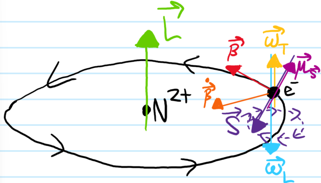
The underlying physics of spin-orbit coupling is neither particularly relativistic nor specific to quantum mechanics. In classical physics, a ball of charge \(q\) and mass \(m\) spinning with angular momentum \(\textbf S\) constitutes a current with magnetic dipole moment \(\boldsymbol{\mu}_{\textbf S}=\gamma\textbf S\) proportional to its spin angular momentum \(\textbf S\) via a proportionality constant \(\gamma=q/2m\) called its gyromagnetic ratio. When placed in an external magnetic field \(\textbf B_{\text{ext}}\), the torque \(\boldsymbol{\tau}=\boldsymbol{\mu}_{\textbf S}\times\textbf B_{\text{ext}}\) experienced by this magnetic dipole causes \(\boldsymbol{\mu}_{\textbf S}=\boldsymbol{\mu}_{\textbf S}(t)\) to precess \(\dot{\textbf S}=\boldsymbol{\omega}_L\times\textbf S\) around the axis \(\boldsymbol{\omega}_L=-\gamma\textbf B_{\text{ext}}\) at the Larmor frequency \(\omega_L=|\boldsymbol{\omega}_L|\). The dipolar potential energy \(V=-\boldsymbol{\mu}_{\textbf S}\cdot\textbf B_{\text{ext}}=\textbf S\cdot\boldsymbol{\omega}_L\) is conserved during the precession.
One should view the spin-orbit coupling of the \(e^-\) as simply taking the classical situation and appending the following relativistic and quantum mechanical paraphernalia:
- The magnetic field \(\textbf B_{\text{ext}}\) is not from some external solenoid, etc. but rather due to the motion of the nucleus \(N^{Z+}\) in the rest frame of the electron \(e^-\). In light of this interpretation, a natural way to compute this magnetic field would be to just Lorentz transform the nuclear Coulomb electrostatic field \(\textbf E_{\text{ext}}=\frac{Z\alpha\hbar c}{e|\textbf X|^2}\hat{\textbf X}\) seen in the lab frame into the magnetic field \(\textbf B_{\text{ext}}=-\frac{1}{\mu c^2}\textbf P\times\textbf E_{\text{ext}}=\frac{Z\alpha\hbar}{e\mu c|\textbf X|^3}\textbf L\) seen in the rest frame of the electron \(e^-\). Alternatively, since one knows that Maxwell’s equations are Lorentz covariant, one can just work directly in the rest frame of the electron \(e^-\), using the Biot-Savart law to compute the magnetic field \(\textbf B_{\text{ext}}(\textbf 0)=\frac{\mu_0\textbf I_N}{2|\textbf X|}\) at the center of the circular current loop due to the orbit of the nucleus \(N^{Z+}\) around the electron \(e^-\) (where \(\mu\) is the reduced mass, not the magnetic dipole moment, and the nuclear current is \(\boldsymbol{\textbf I}_N=\boldsymbol{\mu}_{\textbf L}/\pi|\textbf X|^2=\gamma_{\textbf L}\textbf L/\pi|\textbf X|^2=\frac{g_{\textbf L}Ze}{2\pi m_{N}|\textbf X|^2}\textbf L_N=\frac{g_{\textbf L}Ze}{2\pi\mu|\textbf X|^2}\textbf L\)). It can be checked that these two calculations of the magnetic field \(\textbf B_{\text{ext}}\) agree with each other since \(g_{\textbf L}=1\), though both carry some classical Bohr-like handwaviness.
- \(\gamma\neq q/2m\) but rather \(\gamma_{\textbf S}=g_{\textbf S}q/2m\) where \(q=-e\) and \(g_{\textbf S}\approx 2\) is the spin \(g\)-factor of the electron \(e^-\) (thus, \(\gamma_{\textbf S}<0\) and the electron’s spin and magnetic dipole moment are actually anti-aligned). The fact that \(g_{\textbf S}\neq 1\) is one of the reasons why it is often proclaimed that “spin angular momentum \(\textbf S\) has no classical counterpart” (on this note, it is a common misconception that spin is a purely quantum-mechanical effect. In fact there is no such thing as spin in non-relativistic quantum mechanics. It’s only when one combines quantum mechanics with special relativity that spin emerges in a manner which is not merely ad hoc). Another reason is that such a literal spinning object should also have some rotational kinetic energy \(\textbf S^2/2I>0\) but classically the electron \(e^-\) is a point particle and so has \(I=0\). The effect of this to make the quantum Larmor frequency agree (almost) with the classical cyclotron frequency (some tidal-locking interpretation?).
- In addition to the nuclear magnetic torque inducing the electron’s spin to precess, there is a Coriolis-like competing Thomas torque \(\boldsymbol{\tau}_T=\boldsymbol{\omega}_T\times \textbf S\) trying to make the electron spin precess in the opposite direction, except that it turns out to be only half as strong as the nuclear magnetic torque and so loses this competition (nonetheless, in the absence of such a nuclear magnetic torque, this spin precession would be called Thomas precession). This is a purely kinematic effect of special relativity due to the accumulation of Wigner rotations as one performs non-collinear Lorentz boosts from one instantaneous inertial rest frame to the next instantaneous inertial rest frame in order to “catch up with” the overall non-inertial, rotating frame of the electron \(e^-\). Within the Lorentz group \(O(1,3)\), the Lorentz boosts by themselves do not form a subgroup of \(O(1,3)\) but when combined with spatial rotations, this does form a subgroup, since:
\[\begin{pmatrix}\gamma_2 & -\gamma_2\boldsymbol{\beta}_2^T \\ -\gamma_2\boldsymbol{\beta}_2 & I_3+\frac{\gamma_2^2}{\gamma_2+1}\boldsymbol{\beta}_2\otimes\boldsymbol{\beta}_2\end{pmatrix}\begin{pmatrix}\gamma_1 & -\gamma_1\boldsymbol{\beta}_1^T \\ -\gamma_1\boldsymbol{\beta}_1 & I_3+\frac{\gamma_1^2}{\gamma_1+1}\boldsymbol{\beta}_1\otimes\boldsymbol{\beta}_1\end{pmatrix}=\begin{pmatrix}1 & \textbf 0^T \\ \textbf 0 & R\end{pmatrix}\begin{pmatrix}\gamma_3 & -\gamma_3\boldsymbol{\beta}_3^T \\ -\gamma_3\boldsymbol{\beta}_3 & I_3+\frac{\gamma_3^2}{\gamma_3+1}\boldsymbol{\beta}_3\otimes\boldsymbol{\beta}_3\end{pmatrix}\]
where it is obvious that \(\gamma_3=\gamma_1\gamma_2(1+\boldsymbol{\beta}_1\cdot\boldsymbol{\beta}_2)\) and by taking the trace \(\text{Tr}(R)=1+2\cos\theta\) of \(R\in SO(3)\), one finds that it is associated to a Wigner rotation angle \(\cos\theta=\frac{(1+\gamma_1+\gamma_2+\gamma_3)^2}{(1+\gamma_1)(1+\gamma_2)(1+\gamma_3)}-1\). In particular, when \(\boldsymbol{\beta}_1\cdot\boldsymbol{\beta}_2=0\) are orthogonal as in “circular motion” of the electron \(e^-\) around the nucleus, then \(\gamma_3=\gamma_1\gamma_2\) and the Wigner rotation simplifies to \(\cos\theta=\frac{\gamma_1+\gamma_2}{\gamma_1\gamma_2+1}\). In particular, taking \(\gamma_1=\gamma_{\boldsymbol{\beta}}\) and Taylor expanding \(\gamma_2=\gamma_{\boldsymbol{\beta}+d\boldsymbol{\beta}}\approx\gamma_{\boldsymbol{\beta}}+\gamma_{\boldsymbol{\beta}}^3\boldsymbol{\beta}\cdot d\boldsymbol{\beta}\), one can use the generators of the Lie algebra of the subgroup of \(O(1,3)\) consisting of Lorentz boosts + rotations to show that the Thomas precession angular velocity is (notice the prefactor \(\frac{\gamma^2}{\gamma+1}\) is the same expression appearing in the Lorentz boost matrix):
\[\boldsymbol{\omega}_T=\frac{\gamma^2}{\gamma+1}\boldsymbol{\beta}\times\dot{\boldsymbol{\beta}}\]
Or in the non-relativistic limit \(\gamma\approx 1\):
\[\boldsymbol{\omega}_T\approx \frac{1}{2}\boldsymbol{\beta}\times\dot{\boldsymbol{\beta}}\]
The factor of \(1/2\) is called the Thomas half and cancels out essentially half of the spin-orbit coupling Larmor precession. This is because one just has to replace the previous Larmor frequency with \(\boldsymbol{\omega}_L\mapsto\boldsymbol{\omega}_L+\boldsymbol{\omega}_T\), noting that “Larmor is twice as strong as Thomas” \(\boldsymbol{\omega}_T\approx -\boldsymbol{\omega}_L/2\) (apply Newton’s second law \(\mu\dot{\boldsymbol{\beta}}=-ec\textbf E_{\text{ext}}\) and use the earlier formula for the Lorentz transformation of the nuclear Coulomb electrostatic field \(\textbf E_{\text{ext}}\) into the magnetic field \(\textbf B_{\text{ext}}\)).
Assembling all the ingredients together, one finds the relativistic spin-orbit coupling perturbation to be given by \(\Delta H_{\textbf S\cdot\textbf L}=\beta(|\textbf X|)\textbf S\cdot\textbf L\) as claimed, where the scalar proportionality operator \(\beta(|\textbf X|)=\frac{Z\alpha\hbar(g_{\textbf S}-1)}{2\mu^2c|\textbf X|^3}>0\) is positive-definite so if the electron \(e^-\) is orbiting counterclockwise around the nucleus \(N^{Z+}\), then it will tend to spin clockwise to minimize its spin-orbit coupling energy \(\beta(|\textbf X|)\textbf S\cdot\textbf L\). A picture is worth a thousand words (analogy: the spin angular momentum vector \(\textbf S\) is like a cylinder rolling on a cone).
One can check that \(\textbf S\cdot\textbf L=\frac{1}{2}(S_+L_-+S_-L_+)+S_3L_3\). By observing that the only surviving combinations of ladder operators are \(S_{\pm}L_{\mp}\) and not \(S_+L_+\) or \(S_-L_-\), one is led to the heuristic that if the electron \(e^-\) gains a unit \(\hbar\) of orbital angular momentum \(L_3\) along the \(z\)-axis, then it must lose a unit \(\hbar\) of spin angular momentum \(S_3\) along the \(z\)-axis, and vice versa, in such a way that the total angular momentum \(J_3=L_3+S_3\) along the \(z\)-axis is conserved. To this end, one can regard \(J_3\) as the \(z\)-component of a total angular momentum operator \(\textbf J:=\textbf L+\textbf S\) so that \(\textbf S\cdot\textbf L=\frac{1}{2}(\textbf J^2-\textbf L^2-\textbf S^2)\). In particular, \([H,\textbf J^2]=[H,J_3]=0\) so working in the coupled basis \(|njm_j;\ell s\rangle\) rather than the previously uncoupled basis \(|n\ell sm_{\ell}m_s\rangle\) yields:
\[\textbf S\cdot\textbf L|njm_j;\ell\rangle=\frac{\hbar^2}{2}(j(j+1)-\ell(\ell+1)-s(s+1))|njm_j;\ell\rangle\]
using the fact that the electron is a spin \(s=1/2\) fermion and so by the usual rules of angular momentum addition one has \(m_j=m_{\ell}+m_s\) and \(|\ell-s|\leq j\leq \ell+s\) which is equivalent to \(j=\ell\pm 1/2\) (except for \(\ell=0\) \(s\)-waves where \(j=1/2\) only), this simplifies to:
\[\textbf S\cdot\textbf L|n,j=\ell\pm 1/2,m_j;\ell\rangle=\pm\frac{\hbar^2}{2}\left(\ell+\frac{1}{2}\mp\frac{1}{2}\right)|n,j=\ell\pm 1/2,m_j;\ell\rangle\]
In other words, when the orbital and spin angular momenta are aligned \(j=\ell+1/2\), the spin-orbit coupling energy is \(\sim\hbar^2\ell/2\) whereas when the orbital and spin angular momenta are anti-aligned \(j=\ell-1/2\), then the energy is \(\sim-\hbar^2(\ell+1)/2\), in agreement with the earlier intuition about the anti-aligned configuration being more energetically favorable. In particular, for \(\ell=0\) \(s\)-waves where only the case \(j=1/2\) is relevant, the spin-orbit coupling energy evaluates to \(\hbar^2\times 0/2=0\) so spin-orbit coupling does not affect the ground state(s) \(|100,\pm 1/2\rangle\).
Relativistic Darwin Perturbation
One of the key corollaries of merging special relativity and quantum mechanics is that all the “particles” one is used to such as protons, electrons, etc. are not in fact point particles but rather are smeared out clouds of size \(\lambda\):
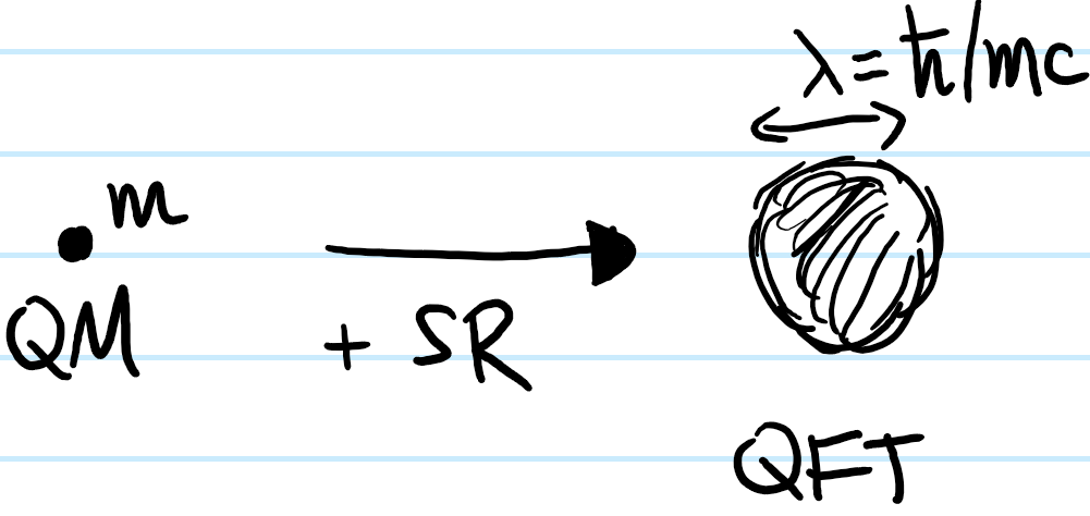
where \(\lambda=\hbar/mc\) is the Compton wavelength of the particle of mass \(m\). Thus for instance, photons \(\gamma\) with \(m_{\gamma}=0\) have \(\lambda_{\gamma}=\infty\) whereas an electron \(e^-\) (which is what one is interested in here) has \(m_{e^-}\sim 10^{-30}\text{ kg}\) and so \(\lambda_{e^-}\sim 10^{-34}/(10^{-30}\times 10^8)\text{ m}\sim 10^{-12}\text{ m}\) (the exact Compton wavelength turns out to be \(\lambda_{e^-}\approx 2.43\times 10^{-12}\text{ m}\)). On these picometer length scales, the electron \(e^-\) no longer looks like a point but rather a swarm of particles and antiparticles. Compared with the Bohr radius \(a_0\approx\lambda_{e^-}/\alpha\), these rapid quantum oscillations (“Zitterbewegung“) are still quite tiny. Consequently, the potential energy of the nucleus \(N^{Z+}\) (which technically also has some nuclear Compton wavelength \(\lambda_N=\lambda_{e^-}\mu/m_N\) except its even shorter than that of the electron \(e^-\) by a factor of \(\mu/m_N\sim 1/1836\), so it is safe to model the nucleus \(N^{Z+}\) as still being a point charge) and the electron \(e^-\) will basically be the same whether one thinks of the electron \(e^-\) as a point charge or as a \(\lambda_{e^-}\)-ball. In the latter case, one roughly expects the electron \(e^-\) to be a distance \(\lambda_{e^-}\) closer to the nucleus \(N^{Z+}\) sometimes, hence experiencing a slightly stronger potential energy \(\sim V(r-\lambda_{e^-})\), but at other times a distance \(\lambda_{e^-}\) further away, experiencing a slightly weaker potential \(\sim V(r+\lambda_{e^-})\) so that heuristically one expects this to just average to \(\sim V(r)\):
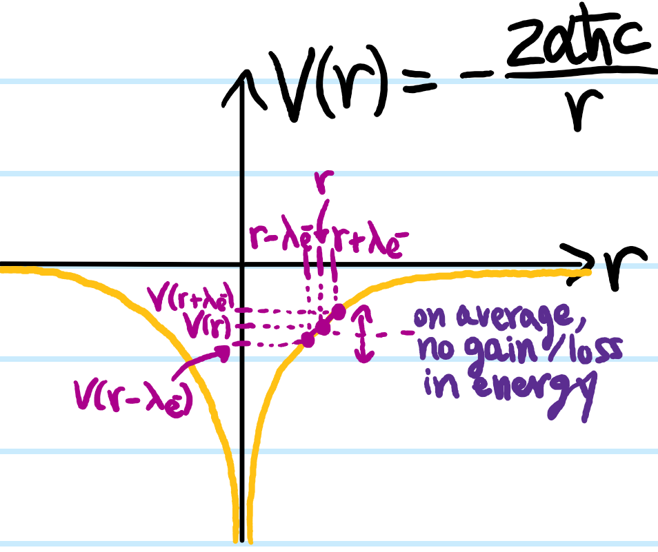
However, there is one point on the diagram where this heuristic clearly fails, namely at the origin \(r=0\) where the nucleus \(N^{Z+}\) rests; here, no matter which direction \(\pm\lambda_{e^-}\) the electron \(e^-\) oscillates, its potential energy \(V(\pm\lambda_{e^-})>V(0)\) can only increase because \(r=0\) is a (global) minimum of the Coulomb potential \(V(r)\) (of course, these arguments are a bit handwavy because \(V(r)\) is actually undefined at \(r=0\)):
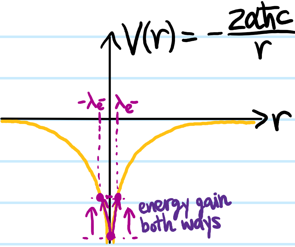
Combined with the fact that Coulomb potential is steepest at \(r=0\), this suggests that only states which can approach the origin \(r=0\) would notice anything. In other words, \(\ell=0\) \(s\)-waves! To formalize this intuition, one can explicitly compute the average Coulomb potential \(\langle V(\textbf x)\rangle_{\lambda_{e^-}}\) in a \(\lambda_{e^-}\)-ball at some position \(\textbf x\in\textbf R^3\):
\[\langle V(\textbf x)\rangle_{\lambda_{e^-}}\sim\frac{1}{\lambda_{e^-}^3}\iiint_{|d\textbf x|\leq\lambda_{e^-}}V(\textbf x+d\textbf x)d^3\textbf x\]
Taylor expanding the integrand (because \(\lambda_{e^-}\) is small):
\[V(\textbf x+d\textbf x)=V(\textbf x)+d\textbf x\cdot\frac{\partial V}{\partial\textbf x}+\frac{1}{2}d\textbf x\cdot\frac{\partial^2 V}{\partial\textbf x^2}d\textbf x+…\]
one sees that the zeroth-order term \(V(\textbf x)\) averages to itself, being just the nuclear Coulomb potential that was in the gross structure Hamiltonian \(H_{\text{gross}}\) all along. The first-order term \(d\textbf x\cdot\frac{\partial V}{\partial\textbf x}\) vanishes upon isotropic averaging. However, the second-order term does not necessarily vanish. It is the averaging of this second-order term which should therefore be treated as the relativistic Darwin perturbation \(\Delta H_{\text{Darwin}}=\frac{1}{2}\langle d\textbf x\cdot\frac{\partial^2 V}{\partial\textbf x^2}d\textbf x\rangle_{\lambda_{e^-}}=\frac{1}{2}\partial_{\mu}\partial_{\nu}V\langle dx^{\mu}dx^{\nu}\rangle_{\lambda_{e^-}}\). For distinct directions \(\mu\neq\nu\) one expects these fluctuations to be uncorrelated, whereas along a given axis \(\mu=\nu\), dimensional analysis asserts that the variance must be of order \(\lambda_{e^-}^2\). However, the exact proportionality constant is not so easy to figure out; a calculation using the Dirac equation shows that the covariance matrix is diagonal with:
\[\langle dx^{\mu}dx^{\nu}\rangle_{\lambda_{e^-}}=\left(\frac{\lambda_{e^-}}{2}\right)^2\delta^{\mu\nu}\]
and therefore, by Poisson’s equation from electromagnetism:
\[\Delta H_{\text{Darwin}}=\frac{\lambda_{e^-}^2}{8}\left|\frac{\partial}{\partial\textbf X}\right|^2V=\frac{Ze^2\hbar^2}{8\mu^2c^2\varepsilon_0}\delta^3(\textbf X)=\frac{\pi Z\alpha\hbar^3}{2\mu^2 c}\delta^3(\textbf X)\]
By virtue of the Dirac delta operator \(\delta^3(\textbf X)\), the relativistic Darwin perturbation only affects states which can approach the origin \(r=0\), again suggesting it only affects \(\ell=0\) \(s\)-waves. This is to be contrasted with spin-orbit coupling which affected all states except for \(\ell=0\) \(s\)-waves.
Fine Structure Corrections to Gross Structure Energies
Having reasoned from physics first principles to derive the relativistic perturbation Hamiltonian:
\[\Delta H_{\text{SR}}=\Delta H_T+\Delta H_{\textbf S\cdot\textbf L}+\Delta H_{\text{Darwin}}\]
where (taking now \(g_{\textbf S}=2\)):
\[\Delta H_T=-\left(\frac{\textbf P^2}{2\mu}\right)^2\frac{1}{2\mu c^2}\]
\[\Delta H_{\textbf S\cdot\textbf L}=\frac{Z\alpha\hbar}{\mu^2c|\textbf X|^3}\textbf S\cdot\textbf L\]
\[\Delta H_{\text{Darwin}}=\frac{\pi Z\alpha\hbar^3}{2\mu^2 c}\delta^3(\textbf X)\]
the task now becomes to calculate how the degeneracy in the gross structure energies \(E_n\) is lifted by these relativistic perturbations \(\Delta H_{\text{SR}}\) to yield the fine structure of the hydrogenic atom. As usual, the eigenspaces of the gross structure Hamiltonian \(H_{\text{gross}}\) are labelled by principal quantum number \(n\in\textbf Z^+\) and have \(2n^2\)-degeneracy as mentioned earlier, so a priori one has to use degenerate perturbation theory. This means one needs to evaluate the matrix elements of \(\Delta H_{\text{SR}}\) restricted to each energy eigenspace \(\ker(H_{\text{gross}}-E_n1)\). Here, the important thing is to choose the right basis for \(\ker(H_{\text{gross}}-E_n1)\) with respect to which one would be calculating the matrix elements of the perturbation \(\Delta H_{\text{SR}}\). Ideally, one would somehow correctly guess an eigenbasis for \(\Delta H_{\text{SR}}\) so that the matrix elements would be trivial to evaluate (all off-diagonal matrix elements would vanish, leaving only expectations on the diagonal so that the different states don’t mix and one is effectively doing non-degenerate perturbation theory). Note that the Wigner-Eckart theorem is useless here because it is not clear how \(\Delta H_{\text{SR}}\) can be interpreted as a component of some spherical tensor operator in the spherical basis. Instead, the idea is contained in the following lemma:
Lemma: Let \(A\) be a Hermitian operator with eigenstates \(|\alpha\rangle, |\alpha’\rangle\) corresponding to distinct eigenvalues \(\alpha\neq\alpha’\in\textbf R\) (hence \(\langle\alpha’|\alpha\rangle=0\)). Suppose that \(A\) commutes with an arbitrary (not necessarily Hermitian) operator \(\Delta H\), i.e. \([A,\Delta H]=0\). Then the off-diagonal matrix element \(\langle\alpha’|\Delta H|\alpha\rangle=0\) vanishes.
Proof: \[0=\langle\alpha’|[A,\Delta H]|\alpha\rangle=(\alpha’-\alpha)\langle\alpha’|\Delta H|\alpha\rangle\]
Thus, here the idea is that one would like to find a complete set of commuting observables (i.e. a set of pairwise-commuting observables with unique simultaneous eigenbasis for the entire state space \(\mathcal H\)) such that as many of the observables in this CSCO also commute with the relativistic perturbation \(\Delta H_{\text{SR}}\). In this case, one can quickly check that:
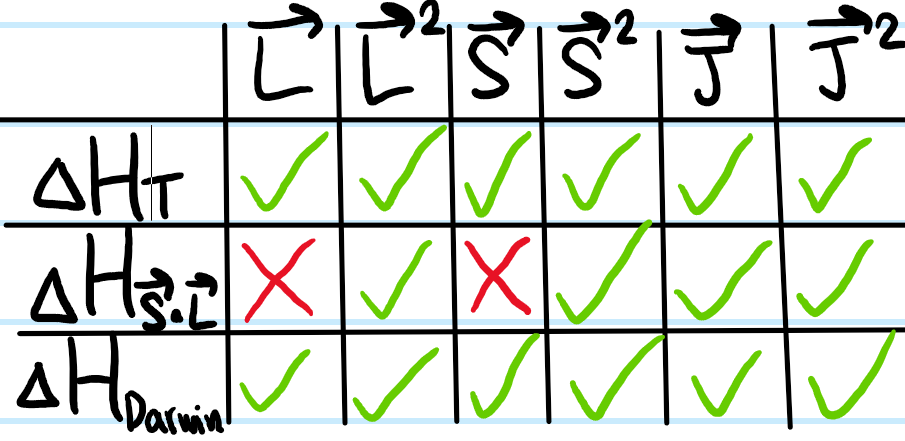
where the green check mark means the two operators commute, the red x if not. It is clear in this case that the CSCO to use is \(\{\textbf L^2,\textbf S^2,\textbf J,\textbf J^2\}\). But this is just the coupled basis \(|njm_j;\ell s\rangle\) mentioned earlier. Working in the uncoupled basis \(|n\ell sm_{\ell}m_s\rangle\) is fine for \(\Delta H_T\) and \(\Delta H_{\text{Darwin}}\) but spin-orbit coupling \(\Delta H_{\textbf S\cdot\textbf L}\) doesn’t like that. Working in the coupled basis makes everyone happy. Degenerate perturbation theory thus reduces to non-degenerate perturbation theory since the coupled basis states don’t mix.
Evaluating the Expectations
The objective is to compute:
\[\langle njm_j;\ell s|\Delta H_{\text{SR}}|njm_j;\ell s\rangle\]
The expectation \(\langle njm_j;\ell s|\Delta H_T|njm_j;\ell s\rangle\) of the relativistic kinetic energy perturbation \(\Delta H_T\) is actually most easily calculated by using Clebsch-Gordan coefficients to rotate back into the uncoupled basis (simply using the resolution of the identity \(|njm_j;\ell s\rangle=\sum_{m_{\ell}m_s}|n\ell sm_{\ell}m_s\rangle\langle\ell sm_{\ell}m_s|jm_j\rangle\) for the ket and similarly for the bra. Note here that the \(s=1/2\) quantum number is being explicitly shown but in practice is often suppressed in the notation because it’s a constant):
\[\langle njm_j;\ell s|\Delta H_T|njm_j;\ell s\rangle=\sum_{m_{\ell}’,m_s’,m_{\ell},m_s}\langle jm_j|\ell sm_{\ell}’m_s’\rangle\langle n\ell sm_{\ell}’m_s’|\Delta H_T|n\ell sm_{\ell}m_s\rangle\langle\ell sm_{\ell}m_s|jm_j\rangle\]
Since \([\Delta H_T,\textbf L]=[\Delta H_T,\textbf S]=0\) (e.g. see the table above), this means \(\Delta H_T\) is a scalar (rank \(0\)) operator with respect to both orbital and spin angular momenta and so by the Wigner-Eckart theorem:
\[\langle n\ell sm_{\ell}’m_s’|\Delta H_T|n\ell sm_{\ell}m_s\rangle=\delta_{m_{\ell}m_{\ell}’}\delta_{m_{s}m_{s}’}\langle n\ell s 0,1/2|\Delta H_T|n\ell s 0,1/2\rangle\]
where the values \(m_{\ell}=0, m_s=1/2\) are arbitrarily chosen for the reduced matrix element (since it doesn’t matter). The computation thus simplifies significantly by virtue of orthonormality \(\sum_{m_{\ell},m_s}\langle j’m_j’|\ell sm_{\ell}m_s\rangle\langle\ell sm_{\ell}m_s|jm_j\rangle=\delta_{jj’}\delta_{m_jm_j’}\) of Clebsch-Gordan coefficients (where here \(j’=j\) and \(m_j’=m_j\)):
\[\langle njm_j;\ell|\Delta H_T|njm_j;\ell\rangle=\langle n\ell s 0,1/2|\Delta H_T|n\ell s 0,1/2\rangle\]
Finally, evaluating the orbital matrix element:
\[\langle n\ell s 0,1/2|\Delta H_T|n\ell s 0,1/2\rangle=-\frac{1}{2\mu c^2}\biggr\langle n\ell s 0,1/2\biggr|\left(\frac{\textbf P^2}{2\mu}\right)^2\biggr|n\ell s 0,1/2\biggr\rangle\]
By writing \(\frac{\textbf P^2}{2\mu}=H_{\text{gross}}-V\), this simplifies to:
\[\langle n\ell s 0,1/2|\Delta H_T|n\ell s 0,1/2\rangle=-\frac{1}{2\mu c^2}(E_n^2-2E_n\langle V\rangle_{n,\ell}+\langle V^2\rangle_{n,\ell})\]
The expectation \(\langle V\rangle_{n,\ell}=2\langle H_{\text{gross}}\rangle_{n,\ell}=2E_n\) is trivial by the virial theorem. However, the expectation \(\langle V^2\rangle_{n,\ell}\) is not so trivial, and requires some mathematical cleverness to evaluate. It turns out to be (and in the circular Rydberg limit \(n\gg 1\), \(\ell=n-1\), agrees with the Bohr model):
\[\langle V^2\rangle_{n,\ell}=(Z\alpha\hbar c)^2\biggr\langle\frac{1}{|\textbf X|^2}\biggr\rangle_{n,\ell}=\left(\frac{Z\alpha}{n}\right)^3\frac{Z\alpha}{\ell+1/2}(\mu c^2)^2\]
Thus, assembling everything together, the first-order correction to the gross structure energies due to the relativistic kinetic energy perturbation \(\Delta H_T\) alone is:
\[\langle n\ell s 0,1/2|\Delta H_T|n\ell s 0,1/2\rangle=-\frac{1}{2}\left(\frac{Z\alpha}{n}\right)^4\left(\frac{n}{\ell+1/2}-\frac{3}{4}\right)\mu c^2<0\]
Now onto spin-orbit coupling. One has (following similar Clebsch-Gordan coefficient manipulations as above and using the earlier results):
\[\langle njm_j;\ell s|\Delta H_{\textbf S\cdot\textbf L}|njm_j;\ell s\rangle=\pm\frac{Z\alpha\hbar^3}{2\mu^2 c}\left(\ell+\frac{1}{2}\mp\frac{1}{2}\right)\biggr\langle\frac{1}{|\textbf X|^3}\biggr\rangle_{n,\ell}\]
Here another bit of mathematical cleverness (using the scalar radial momentum operator \(P_r:=(\hat{\textbf X}\cdot\textbf P+\textbf P\cdot\hat{\textbf X})/2\) to derive the Kramers-Pasternack recurrence relations) is needed to show that:
\[\biggr\langle\frac{1}{|\textbf X|^3}\biggr\rangle_{n,\ell}=\frac{1}{\ell(\ell+1/2)(\ell+1)}\left(\frac{Z}{na_0}\right)^3\]
So that the first-order correction to the gross structure energies due to spin-orbit coupling is:
\[\langle n,j=\ell\pm 1/2,m_j;\ell s|\Delta H_{\textbf S\cdot\textbf L}|n,j=\ell\pm 1/2,m_j;\ell s\rangle=\pm\frac{1}{2}\left(\frac{Z\alpha}{n}\right)^4\frac{n}{(\ell+1/2\pm 1/2)(\ell+1/2)}\mu c^2\]
Finally, for the relativistic Darwin term, using the same kinds of arguments as above, one finds (using \(\langle\textbf 0|n\ell sm_{\ell}m_s\rangle=\frac{2}{\sqrt{4\pi}}\left(\frac{Z}{na_0}\right)^{3/2}\delta_{\ell,0}\)) that:
\[\langle njm_j;\ell s|\Delta H_{\text{Darwin}}|njm_j;\ell s\rangle=\delta_{\ell,0}\frac{1}{2}\left(\frac{Z\alpha}{n}\right)^4n\mu c^2>0\]
Assembling all energy corrections together, one finally obtains the net first-order relativistic correction to the gross structure energies:
\[\langle njm_j;\ell s|\Delta H_{\text{SR}}|njm_j;\ell s\rangle=\frac{Z^2\alpha^2E_n}{n}\left(\frac{1}{j+1/2}-\frac{3}{4n}\right)<0\]
there are \(2\) miracles that have happened here. The first is that, for \(\ell>0\), the above formula is the result one would obtain regardless of whether \(j=\ell\pm 1/2\) (an accidental degeneracy in this context, though actually natural if one starts from the Dirac equation). The second miracle is that, when \(\ell=0\), the spin-orbit coupling correction should actually vanish, but then the Darwin correction kicks in and adds back exactly what spin-orbit coupling would have added, so that the final formula is valid for all \(\ell\in\textbf N\) and \(j=\ell\pm 1/2\) (remembering that for \(\ell=0\) one only has \(j=1/2\)). This should be compared with the “exact” expression at the level of fine structure given by the Dirac equation:
\[E_{n,j}=-\mu c^2\left[1-\left(1+\left[\frac{Z\alpha}{n-j-1/2+\sqrt{(j+1/2)^2-(Z\alpha)^2}}\right]^2\right)^{-1/2}\right]\]
Thus, at a high level, after spin-orbit coupling was introduced, \(m_{\ell},m_s\) were no longer good quantum numbers (but \(n,\ell,s\) still were), so had to be replaced by two new good quantum numbers \(j,m_j\). These fine structure corrections actually failed to lift the \(\ell\)-degeneracy, but nevertheless there is now a \(j\)-dependence which wasn’t there at the level of the gross structure.
Comments about notation \(n\ell_j\) and degeneracy of states in \(n\ell_j=\sum_{j=\ell\pm 1/2}(2j+1)\)?
Hyperfine Structure of Hydrogenic Atoms
Just as the fine structure of hydrogenic atoms was obtained from special relativity, one could roughly say that the hyperfine structure of hydrogenic atoms comes from quantum chromodynamics, or more simply, from no longer treating the nucleus \(N^{Z+}\) as just a point charge \(Ze\) at the origin, but rather having some internal structure to it as well. In other words, it turns out (because protons \(p^+\) and neutrons \(n^0\) are spin-\(1/2\) fermions just like the electron \(e^-\)) that the nucleus \(N^{Z+}\) also has some spin angular momentum \(\textbf I:=\textbf S_{N}\) which gives rise to a nuclear magnetic dipole moment \(\boldsymbol{\mu}_{\textbf I}=\gamma_{\textbf I}\textbf I\) where now the nuclear gyromagnetic ratio is \(\gamma_{\textbf I}=\frac{g_{\textbf I}Ze}{2m_N}\). There are \(2\) other angular momenta that the nuclear spin angular momentum \(\textbf I\) can couple to, namely the orbital angular momentum \(\textbf L\) of the electron \(e^-\) and its spin angular momentum \(\textbf S\). These lead respectively to nuclear perturbations \(\Delta H_N=\Delta H_{\textbf I\cdot\textbf L}+\Delta H_{\textbf I\cdot\textbf S}\) to the fine structure Hamiltonian \(H_{\text{HFS}}=H_{\text{FS}}+\Delta H_N\) given respectively by:
\[\Delta H_{\textbf I\cdot\textbf L}=\beta(|\textbf X|)\textbf I\cdot\textbf L\]
\[\Delta H_{\textbf I\cdot\textbf S}=-\frac{\mu_0}{4\pi|\textbf X|^3}[3(\boldsymbol{\mu}_{\textbf I}\cdot\hat{\textbf X})(\boldsymbol{\mu}_{\textbf S}\cdot\hat{\textbf X})-\boldsymbol{\mu}_{\textbf I}\cdot\boldsymbol{\mu}_{\textbf S}]-\frac{2\mu_0}{3}\boldsymbol{\mu}_{\textbf I}\cdot\boldsymbol{\mu}_{\textbf S}\delta^3(\textbf X)\]
The former is just spin-orbit coupling but now in the rest frame of the nucleus (which is normally one how thinks about hydrogenic atoms anyways). The second is just the standard formula from electromagnetism for the interaction energy between two dipoles due to their intrinsic magnetic fields. Although normally one wouldn’t really care about the \(\delta^3(\textbf X)\) term since one is typically interested in the far-field behavior of the magnetic field, actually here it turns out to be crucial! Finally, note that sometimes the electric quadrupole moment (NOT a magnetic quadrupole moment) of the nucleus \(N^{Z+}\) and its interaction with the non-uniform electric (not magnetic!) field of the electron \(e^-\) is also counted as a hyperfine effect, but here it will just be ignored.