
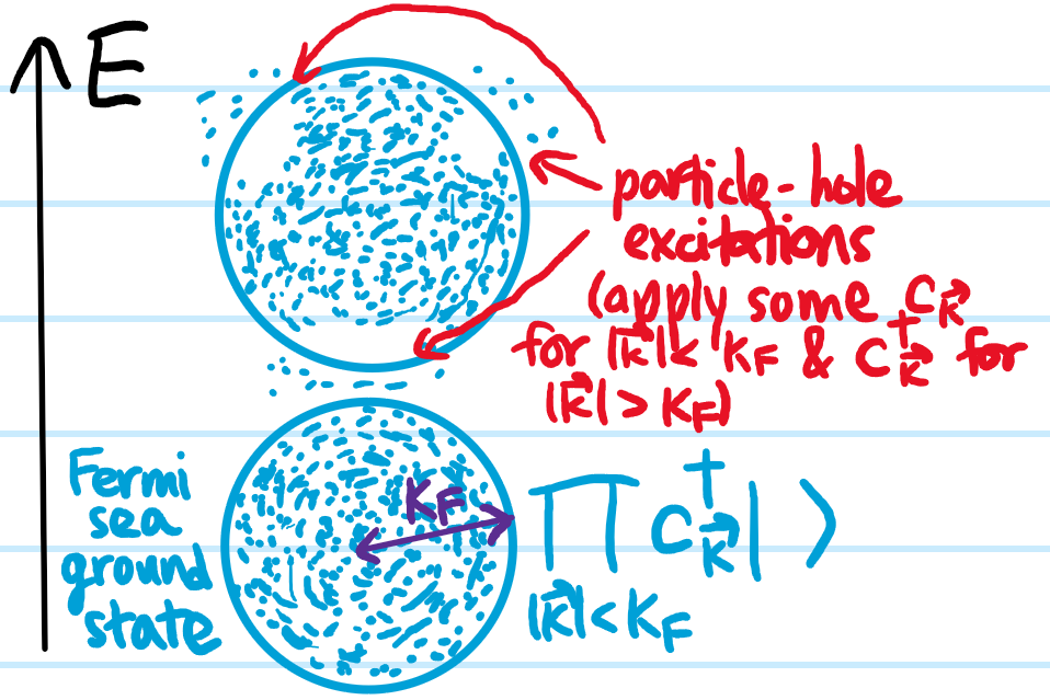
Problem: What is the meant by the phrase “elementary excitations” of an ideal Fermi gas?
Solution: Basically “excitations” is a fancy word for “excited states”, in this case more precisely “many-body excited states”. One example is depicted in the diagram below. Note that the elementary excitations are the subset of all excitations involving only a single fermion creation/annihilation operator (i.e. only removing \(1\) fermion from the Fermi sea, or only adding \(1\) fermion to a state beyond the Fermi sea; thus particle-hole excitations are not elementary excitations but could be thought of as composed of \(2\) elementary excitations).
Problem: What is a rule of thumb for the difference between quasiparticles and collective excitations?
Solution: Quasiparticles (e.g. holes) are fermionic while collective excitations (e.g. phonons) are bosonic.
Problem: Define an adiabatic process in quantum mechanics.
Solution: It needs to go sufficiently slow (similar to the notion of quasistatic (indeed, reversible) process in thermodynamics, and unfortunately the exact opposite of what “adiabatic” means in thermo). This ensures that one can describe a well-defined evolution of the eigenenergies of the eigenstates as a function of the adiabatic turn-on of the interaction potential (again, analogous to thermo, quasistatic is needed to define the set of equilibrium states connected tgt). In particular, provided the states are separated from each other, then the adiabatic theorem guarantees there will not be a level crossing; \(E_1(\lambda=0)<E_2(\lambda=0)\Rightarrow E_1(\lambda)<E_2(\lambda)\) for all \(\lambda\in[0,1]\) which at the macroscopic level is equivalent to saying there will not be a phase transition (e.g. if ground state were to swap). Note the adiabatic theorem applies to the \(N\)-particle sector of the Fock space, and specifically to the many-body eigenstates (not single-particle eigenstates), and also in FLT, calling it “adiabatic principle” is a misnomer, should just be called “adiabatic assumption”.
Given a many-body interacting system of identical fermions, explain the necessary (but not sufficient) condition of adiabaticity that the fermion interactions must fulfill in order for that system of identical fermions to deserve the name/classification of being a “Fermi liquid“.
Solution: A Hamiltonian \(H\) is said to be adiabatically connected to another Hamiltonian \(H_0\) iff there exists a smooth path in “Hamiltonian space” from \(H_0\to H\). Here “smooth” means no level crossings of the eigenstates, or \(\Leftrightarrow\) no phase transitions. Also, just as in thermodynamics when one sketches e.g. an isotherm or adiabat on a \(pV\)-diagram which is always implicitly showing a quasistatic and in fact reversible process connecting a bunch of equilibrium states together, so here too the “path” in Hamiltonian space should be traversed sufficiently slowly as a function of time \(t\) (as quantified for instance by the adiabatic theorem). Of course in the lab, the interactions in \(H\) are already “on”, so this rather technical minutiae is at best a gedankenexperiment.
A system of identical fermions with interacting Hamiltonian \(H\) only has any hope of being a Fermi liquid if \(H\) is adiabatically connected to the corresponding non-interacting Hamiltonian \(H_0\) of an ideal Fermi gas as a reference system. In other words, from a topological/phase diagram perspective, Fermi liquids are a subset of the connected component of the ideal Fermi gas.
The “meaty corollary” that adiabaticity brings with it as that, if it’s satisfied, then there must exist a bijection between the ideal Fermi gas and the interacting Fermi liquid. The essence of theoretical physics is to map hard problems to easy problems! And moreover, these sorts of isomorphisms reveal a lot of deep connections/symmetries (e.g. in this case experiments found linear heat capacities, constant Pauli diamagnetism, etc. which were predicted qualitatively in the ideal Fermi gas model despite interactions…this isomorphism is the essence of Landau’s explanation of that remarkable observation).
The “rigorous proof” of this isomorphism goes back to the gedankenexperiment above, i.e. that it should be possible to “trace the footsteps” of each non-interacting eigenstate \(N_{\textbf k}\) of \(H_0\) through state space to end up at the unique, corresponding eigenstate of \(H\).
Henceforth, write \(\tilde N_{\textbf k}\) to denote the eigenstate of the interacting fermion system \(H\) adiabatically connected to \(N_{\textbf k}\); note that \(N_{\textbf k}\neq \frac{1}{e^{\beta (E_{\textbf k}-\mu)}+1}\) can be any arbitrary, possibly non-equilibrium occupation number distribution in \(\textbf k\)-space, so long as it’s compatible with Pauli exclusion \(N_{\textbf k}\in\{0,1\}\). This is roughly saying that “eigenvalues are more robust than eigenvectors” with respect to perturbations, or in quantum lingo, “quantum numbers are more robust than eigenstates”; although \(\textbf k\) in general will no longer be a good quantum number for basically any kind of interactions, one can sort of “pretend” that it’s a good quantum number anyway by using it as an adiabatic label for the interacting eigenstates of \(H\).
Problem: (something about the ansatz…)
Solution: For a degenerate ideal Fermi gas, the occupation numbers are given by a sharp Fermi-Dirac step \(N_{\textbf k}=\Theta(k_F-|\textbf k|)\) and the total energy is \(E=\frac{3}{5}NE_F\). Now suppose one were to shuffle the fermions around in \(\textbf k\)-space, effectively moving some fermions from the \(|\textbf k|<k_F\) Fermi sea (leaving behind holes) and promoting them to the unoccupied region \(|\textbf k|>k_F\). Then within the \(|\textbf k|<k_F\) Fermi sea, if a fermion was removed from a particular \(\textbf k\)-state, then the occupation number \(N_{\textbf k}\) of that \(\textbf k\)-state will have decreased by \(\Delta N_{\textbf k}=-1\). Similarly, if that fermion is then added to a \(\textbf k\)-state outside the Fermi sea \(|\textbf k|>k_F\), the occupation number of that \(\textbf k\)-state would increase by \(\Delta N_{\textbf k}=1\). It is thus clear that the total energy of the degenerate ideal Fermi gas would increase from its initial value of \(E=\frac{3}{5}NE_F\) by an amount:
\[\Delta E=\frac{\textbf k}\frac{\hbar^2|\textbf k|^2}{2m}\Delta N_{\textbf k}\]
where the sum \(\sum_{\textbf k}\) is of course over all \(\textbf k\)-states, both inside and outside the Fermi sea (and due to the monotonically increasing nature of the free particle dispersion \(\sim|\textbf k|^2\), the positive contributions from outside the Fermi sea will necessarily overwhelm the negative contributions from within the Fermi sea leading to an increase \(\Delta E>0\) as mentioned above).
So far this discussion has been for a ideal (aka non-interacting) Fermi gas. What happens if the fermions can now interact with each other (e.g. Coulombic repulsion between electrons)? Then Landau postulated that the above expression should be replaced by:
\[E=\sum_{\textbf k,\sigma}\frac{\hbar^2}{m^*}k_F(k-k_F)\delta N_{\textbf k}+\frac{1}{2}\sum_{\textbf k,\textbf k’,\sigma,\sigma’}f_{\textbf k,\textbf k’,\sigma,\sigma’}\delta N_{\textbf k,\sigma}\delta N_{\textbf k’,\sigma’}\]
Problem: Show that for \(T\ll T_F\) and \(E-\mu\ll\mu\), the quasiparticle lifetime \(\tau\) goes like:
\[\tau=\frac{\hbar\mu}{a(E-\mu)^2+b(k_BT)^2}\]
for dimensionless constants \(a,b\in\textbf R\) of \(O(1)\). In particular, for a \(T=0\) degenerate Fermi liquid, one has \(\tau\sim 1/(E-E_F)^2\) so the closer the energy \(E\) of the quasiparticle is to the Fermi energy \(E_F\), the longer-lived it is.
Solution: This can be obtained simply from an application of Fermi’s golden rule to the (obviously dominant!) scattering process of a quasiparticle with momentum \(|\textbf k|>k_F\) colliding with a Fermi sea particle of momentum \(|\textbf k_2|<k_F\) and ending up as \(2\) quasiparticles outside the Fermi sea \(|\textbf k’_1|,|\textbf k’_2|>k_F\). This decay channel is obviously dominant because of Pauli blocking (what else could possibly happen?) and is enforced by the corresponding step functions (each either \(0,1\)) in the density of final states:
\[\frac{1}{\tau_{\textbf k}}=\frac{2\pi}{\hbar}\sum_{\textbf k_2,\textbf k’_1,\textbf k’_2}|\langle\textbf k’_1,\textbf k’_2|V|\textbf k,\textbf k_2\rangle|^2\Theta(k_F-|\textbf k_2|)(1-\Theta(k_F-|\textbf k’_1|))(1-\Theta(k_F-|\textbf k’_2|))\delta_{\textbf k+\textbf k_2,\textbf k’_1+\textbf k’_2}\delta_{E_{\textbf k}+E_{\textbf k_2},E_{\textbf k’_1}+E_{\textbf k’_2}}\]
(aside: are the assumptions of Fermi’s golden rule sufficiently fulfilled in this case?). Actually, if we want to extract the \(T\)-dependent part of \(\tau_{\textbf k}\), then instead of step functions we should linearize Fermi-Dirac at temperature \(T\) about the Fermi surface. Justify that this is because in fact, with a little thought (can be proven mathematically), all of the wavevectors actually need to be pretty close to the Fermi surface for momentum and kinetic energy constraints to be satisfiable.
Problem: What are \(2\) examples of quantum systems to which Landau’s Fermi liquid theory applies?
Solution: Normal (i.e. not superfluid) \(^3\text{He}\) and normal (i.e. not superconducting) conduction electrons in a conductor (the latter case has a bit more complications due to the long-range nature of the Coulomb electrostatic repulsion whereas in He-3 it’s just short-range VdW LJ).
References:
https://www.cambridge.org/core/books/abs/statistical-mechanics-and-applications-in-condensed-matter/fermi-liquids/6BB91EF8A8EB8E2AA7F7630D341C5234
https://www.cambridge.org/core/books/abs/quantum-theory-of-the-electron-liquid/normal-fermi-liquid/59F1693E7C95315DF101D2D492BF7386
https://www.cambridge.org/core/books/abs/advanced-quantum-condensed-matter-physics/landau-fermi-liquid-theory/A56792EFE45087D87EA48F578B50D719
https://www.cambridge.org/core/books/abs/ultracold-atomic-physics/fermi-liquid/A04490E00A1B276F7FEB888D2902AF9E
https://www-thphys.physics.ox.ac.uk/people/SteveSimon/QCM2019/QuantumMatterApr30.pdf